FEM Electromagnetics in Python: A Complete Ecosystem Guide
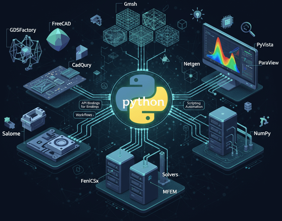
Navigate the open-source Python ecosystem for electromagnetic simulation, from geometry creation with GDSFactory and FreeCAD to solving with Palace and FEniCSx, and visualization with PyVista.

If you’re venturing into computational electromagnetics with open source tools, you’ve probably noticed something: the landscape is fragmented. Unlike commercial EM packages that bundle everything from geometry creation to field visualization, the open source world offers specialized tools that excel at specific aspects of electromagnetic simulation.
The good news? Python has emerged as the universal glue that binds these tools into coherent EM workflows. This guide will help you navigate this ecosystem and understand how these pieces fit together for antenna design, photonics, waveguide analysis, and RF engineering.
The Python Philosophy: Glue, Don’t Reinvent
Before diving into specific tools, it’s worth understanding why Python dominates this space. Python isn’t the fastest language for number crunching—that’s why solvers are written in C++, Fortran or Julia. But Python excels at glueing tools together, and has by far the largest open-source ecosystem. If there is a specialized C++ tool that could fit into your CAD/CAE workflow, chances are that someone has already built Python bindings for it, and some convenience tool on top.
There are already Python tools that let you:
- Generate geometries programmatically
- Control meshing parameters without GUI clicking
- Launch EM simulations with varied parameters (frequency sweeps, material properties, geometry variations)
- Post-process field results with the same script that set up your antenna or waveguide problem
- Integrate disparate tools that were never designed to work together
Let’s dig deeper into the different stages of a typical electromagnetic simulation workflow and see what the open-source ecosystem (and in particular, the Python ecosystem) has to offer.
The Geometry and Meshing Landscape
Your first major decision involves geometry creation and meshing for electromagnetic structures. You’ll primarily encounter three approaches: FreeCAD, Gmsh, and Salome, as well as some notable specialized variants like CadQuery and domain-specific tools like GDSFactory for photonics and quantum RF.
Before diving into specifics, it’s worth noting what unites most of these tools under the hood: OpenCascade (OCCT), the open source CAD kernel that powers FreeCAD, Gmsh, and Salome. OpenCascade handles the underlying geometric operations (booleans, filleting, NURBS surfaces) that make solid modeling possible. This shared foundation means geometries created in one tool can generally be understood by another, and explains why you’ll see similar capabilities (and occasionally similar quirks) across the ecosystem.
GDSFactory takes a different approach, using pure Python geometry primitives optimized for planar structures, which makes it exceptionally efficient for generating complex layouts. In fact, GDSFactory has emerged as the standard Python framework for photonic integrated circuit design and quantum RF applications, enabling reproducible, version-controlled layouts with seamless integration into simulation workflows. Its programmatic approach to geometry generation makes it particularly powerful for parameter sweeps and optimization studies in both photonics and quantum RF circuit design.
The Metadata Problem
You might define a “copper” conductor with specific conductivity and assign it to certain faces in FreeCAD, or set up a “perfect electric conductor” boundary condition on antenna surfaces, but when you export the mesh to a solver like Palace or FEniCSx, that information doesn’t automatically transfer. You’ve got geometry and connectivity, but the EM physics metadata is gone. Now you need to either:
- Re-identify those regions in the solver (error-prone for complex antenna geometries)
- Develop custom export/import scripts that carry EM metadata through your toolchain
- Use naming conventions and tags that survive the export process
Different tools handle this differently. Some use physical groups (Gmsh), some use named selections (Salome), some embed data in mesh formats (XDMF), and some require you to build the connection manually. There’s no universal standard, which means every tool transition in your workflow is a potential point where electromagnetic material properties and boundary conditions can be lost or corrupted. This is particularly painful for EM applications where you might have multiple dielectric materials, frequency-dependent losses, and complex boundary conditions like ports or absorbing boundaries.
Integration Strategies: Choosing Your Tools
Each tool in the geometry and meshing landscape offers different tradeoffs. Here’s how to choose and integrate them effectively.
FreeCAD: Parametric CAD with Integrated FEM
FreeCAD deserves special attention because of its generality as a CAD engine, modular design and extensibility. It bridges worlds that often don’t communicate. It’s a parametric CAD system — think feature-based modeling like SolidWorks or Fusion 360, but open source. You can design parts with sketches, extrudes, and fillets, all while maintaining a design history tree. Its Python API exposes the entire CAD kernel:
import FreeCAD
import Part

box = Part.makeBox(10, 10, 10)
sphere = Part.makeSphere(7)
result = box.cut(sphere)
But FreeCAD goes further with its FEM Workbench, which integrates meshing (via Gmsh and Netgen) and solving (via CalculiX and Elmer) directly in the interface. For RF engineers transitioning from commercial CAD/EM packages, this feels familiar—define antenna geometry, assign conductor/dielectric materials, set up boundary conditions, mesh, solve, visualize.
The FEM Workbench’s real value isn’t replacing specialized EM solvers; it’s providing a framework that keeps material properties and boundary conditions connected to geometry throughout the workflow. You can set up EM analysis without leaving FreeCAD, but a professional use requires integrating specialized EM solvers like Palace into FreeCAD, which is doable but can be challenging. The Python console and macro system will let you automate the entire workflow, making parameter sweeps straightforward.
In sum, consider FreeCAD if you are interested in an integrated FEM environment that can potentially sidestep many metadata problems.
Gmsh: Excellent Meshing with Clean Python API
Gmsh remains a popular choice for its excellent meshing algorithms and exceptionally clean Python API. While it includes OpenCascade-based geometry capabilities, many users import geometries from other tools and use Gmsh purely for meshing—and that’s where it truly shines. Its meshing algorithms are among the best in the open source world, handling everything from simple 2D shapes to complex 3D volumes with both structured and unstructured approaches.
The key insight with Gmsh is its “physical groups” system. Unlike raw mesh files that just contain vertices and connectivity, Gmsh lets you tag regions and boundaries with meaningful names. Define a “copper_patch” physical surface or a “dielectric_substrate” physical volume, and these tags export with the mesh. This helps preserve critical metadata through the pipeline—though it requires careful bookkeeping since you’re defining these groups based on geometric entities.
import gmsh

gmsh.initialize()
gmsh.model.add("waveguide")

# Create geometry
rect = gmsh.model.occ.addRectangle(0, 0, 0, 10, 5)
gmsh.model.occ.synchronize()

# Define physical groups for EM simulation
gmsh.model.addPhysicalGroup(2, [rect], 1)
gmsh.model.setPhysicalName(2, 1, "waveguide_cross_section")

gmsh.model.mesh.generate(2)
gmsh.write("waveguide.msh")
gmsh.finalize()
The Python API is remarkably comprehensive—you can script the entire geometry-to-mesh pipeline without touching the GUI. This makes Gmsh perfect for automated workflows, parameter sweeps, and integration into larger simulation chains. Need to mesh 100 antenna variations? Write a loop in Python. Want to integrate meshing into a CI/CD pipeline? Gmsh handles it elegantly.
For EM workflows, Gmsh integrates particularly well with solvers like Palace and FEniCSx. The physical groups you define translate cleanly to boundary conditions and material regions. The challenge is maintaining the connection between your EM intent and the geometric tagging—you need to carefully track which surface IDs correspond to ports, which volumes are dielectrics, and which boundaries need absorbing conditions.
In sum, use Gmsh when you want minimal dependencies, excellent mesh quality, and need to integrate meshing into larger automated workflows.
Salome: Comprehensive Pre-Processing Platform
Salome represents the opposite philosophy from Gmsh’s focused simplicity—it’s a complete CAD and pre-processing platform that aims to handle everything from geometry creation through mesh generation to solver setup. Think of it as an open source alternative to commercial pre-processors like Ansys Workbench, but with full Python scriptability.
Salome’s strength lies in handling complex, real-world CAD assemblies. When you receive a STEP file from mechanical engineers containing an entire antenna system with mounting brackets, RF connectors, and housing—complete with all the messy details of real engineering models—Salome has the tools to handle it. It includes sophisticated geometry healing algorithms to fix common CAD import issues (broken surfaces, tolerance mismatches, duplicate entities), Boolean operations that work reliably on complex shapes, and advanced meshing algorithms that can handle challenging geometries.
The Python interface (called TUI - Text User Interface) gives scriptable access to Salome’s entire feature set. Unlike some tools where the GUI and scripting are separate, Salome’s GUI actually generates Python code, which you can capture and reuse:
import salome
salome.salome_init()

from salome.geom import geomBuilder
geom = geomBuilder.New()

# Import CAD and perform healing
antenna_assembly = geom.ImportSTEP("antenna_housing.step", True, True)
healed = geom.RemoveExtraEdges(antenna_assembly, True)

# Create mesh with different element sizes for different regions
from salome.smesh import smeshBuilder
mesh = smeshBuilder.New()
antenna_mesh = mesh.Mesh(healed)

# Define algorithms and parameters
mesh.Triangle().MaxElementArea(1.0)
mesh.AutomaticHexahedralization()
mesh.Compute()

# Export with named groups
mesh.ExportMED("antenna_mesh.med")
For EM workflows, Salome’s named selections and group management become crucial when dealing with complex geometries. You can select surfaces by color, material name, or geometric properties, then assign them to named groups that carry through to the solver. This is particularly valuable when importing industrial CAD where material assignments might already be embedded in the file structure.
The learning curve is real—Salome is a complete simulation environment, not just a meshing tool. You’re learning multiple modules (Geometry, Mesh, sometimes ParaVis for visualization), each with their own concepts and workflows. But for complex industrial workflows, especially those involving imported CAD from other engineering teams, this comprehensiveness becomes necessary rather than burdensome.
In sum, turn to Salome when you’re dealing with complex CAD assemblies, multi-scale geometries (IC packages to full antenna systems), or need sophisticated geometry healing for real-world CAD imports. It’s the tool that bridges the gap between idealized textbook geometries and messy industrial reality.
Solving: Choosing Your Framework
Once you have your geometry meshed and ready, the next critical decision is choosing the right solver framework. This is where paths diverge based on your specific electromagnetic physics needs. While the geometry and meshing tools we discussed are relatively universal across simulation domains, EM solvers are highly specialized—optimizing for different frequency regimes, problem types, and computational approaches. Your choice here will significantly impact not just performance, but the types of problems you can tackle and how naturally you can express your physics.
General-Purpose FEM: FEniCSx
If you’re solving custom electromagnetic PDEs — whether implementing novel metamaterial models, multiphysics EM-thermal coupling, or research-level EM problems — FEniCSx (the successor to FEniCS) deserves serious consideration. It’s a complete finite element framework where you express Maxwell’s equations in near-mathematical notation:
from dolfinx import fem, mesh
# Define Maxwell's equations weak form almost as you'd write it on paper
a = inner(curl(E), curl(v)) * dx - k0**2 * inner(eps * E, v) * dx
FEniCSx handles the discretization, assembly, and solving. It’s particularly elegant for custom EM physics or coupled problems (EM-thermal, EM-mechanical). The learning curve is real—you need to understand variational formulations of Maxwell’s equations—but the payoff is flexibility. You’re not limited to pre-defined EM modules and can implement cutting-edge EM research directly.
The recent FEniCSx rewrite improved performance and parallel scalability significantly. If your problems are getting large or you’re running on HPC clusters, this matters.
Electromagnetic-Specific FEM: Palace
Electromagnetic simulations have unique requirements, and Palace addresses them directly. Built on MFEM, Palace provides a domain-specific solver for EM problems — eigenmode analysis, frequency domain, time domain—without requiring you to implement Maxwell’s equations from scratch.
Palace’s Python interface lets you configure complex EM scenarios, manage material properties, and set up boundary conditions programmatically. It’s particularly strong for RF cavities, waveguides, and antenna problems. The advantage over general-purpose tools is that EM-specific features (ports, periodic boundaries, eigenvalue solvers tuned for Maxwell’s equations) are built in.
An Integrated Approach: Emerge
Emerge represents a different philosophy: purpose-built integration for specific workflows. Rather than being a general-purpose tool, Emerge targets specific use cases with tighter end-to-end integration.
Notably, Emerge developed its own CAD mini-language (similar to tools like CadQuery) that lets you define geometries programmatically while simultaneously tagging material properties and boundary conditions directly in the geometry definition. This addresses the metadata problem head-on—your physics information is embedded from the start, not added later and potentially lost during export.
The tradeoff is scope and performance. Emerge isn’t designed for high-performance computing or solving extremely large problems. It’s optimized for specific workflows where the integration value outweighs raw computational power. If your problems fit within Emerge’s performance envelope and align with its target applications, the reduced friction can be significant.
This exemplifies a broader pattern in the ecosystem: highly integrated tools trade generality and performance for workflow simplicity. Commercial CAE packages do this too—they bundle everything so you don’t have to integrate, but you’re limited to their choices. Emerge makes similar tradeoffs within the open source world.
Post-Processing: Making Sense of Your Results
Visualization: PyVista and ParaView
You’ve run your simulation. Now you’re staring at gigabytes of data. This is where PyVista becomes indispensable.
PyVista wraps VTK (the Visualization Toolkit) in a Pythonic interface that doesn’t make you want to tear your hair out. Want to plot a scalar field on a mesh? It’s actually intuitive:
import pyvista as pv

mesh = pv.read('results.vtu')
mesh.plot(scalars='temperature', cmap='hot')
But PyVista’s real value is integration. You can read mesh data, manipulate it, compute derived quantities, and visualize—all in the same script that set up your simulation. Need to extract data along a line? Compute gradients? Generate animations? It’s all scriptable.
For interactive exploration, ParaView remains king. While you can script ParaView with Python (and should, for reproducible visualization), sometimes you need to click around, try different colormap ranges, and explore your data interactively. ParaView’s power comes from its filters (clip, slice, threshold, streamlines) that you can chain together.
The workflow many adopt: Use ParaView interactively to figure out what visualizations tell the story, then script those exact operations with PyVista for reproducibility and batch processing.
Building Your Workflow: Python as Glue
Here’s where everything comes together. A typical scripted EM workflow might look like:
- Generate geometry (Gmsh API, GDSFactory for plannar circuits, or FreeCAD Python)
- Mesh with EM-appropriate elements (Gmsh, Netgen, or Salome meshing with proper edge elements)
- Export to EM solver format (various mesh I/O libraries, preserving EM boundary conditions)
- Run EM simulation (Palace, FEniCSx for custom EM PDEs, femwell for photonics, etc)
- Post-process EM fields (PyVista for field visualization, NumPy/SciPy for S-parameters, far-field calculations)
All in one Python script. Change an antenna parameter, frequency, or material property at the top, rerun, and everything updates. This is the power of Python as glue for EM workflows. For photonics applications, GDSFactory particularly excels at generating complex device layouts that can then flow seamlessly into simulation pipelines.
Practical Integration Tips
Format compatibility matters. Invest time in understanding mesh formats (MSH, XDMF, VTU) and how they handle EM-specific data like edge elements, material properties, and boundary conditions. Tools like meshio (a Python library) can convert between formats, saving you from manual conversions.
Version control your scripts, not your field results. Your Python EM workflow script should be able to regenerate any S-parameter, far-field pattern, or field plot. This is reproducibility in practice for EM simulations.
Start with simple EM problems. Before building elaborate antenna optimization pipelines, make sure you can run each tool independently. Get a simple waveguide meshed in Gmsh. Solve a basic EM eigenmode problem in Palace. Visualize electric field patterns in PyVista. Then connect them.
Embrace notebooks for EM exploration, scripts for production. Jupyter notebooks are excellent for developing antenna designs and documenting EM workflows. But for frequency sweeps, parameter optimization, or HPC EM runs, convert to scripts.
Which Path Should You Take?
If you’re an RF engineer working with mechanical teams on antenna integration: FreeCAD’s FEM Workbench provides the lowest friction path for combining mechanical CAD with EM analysis. You can design antenna housings, analyze mechanical constraints, and perform EM simulations in one environment. Perfect for antenna placement or antenna tunning studies or when you need to communicate with mechanical engineers using familiar CAD paradigms.
If you’re focused on waveguide analysis, cavities, or high-frequency structures: Palace (built on MFEM) provides production-grade EM simulation with excellent eigenmode analysis and frequency-domain capabilities. The Palace + PyVista combination handles everything from microwave filters to accelerator cavities with proper handling of ports, periodic boundaries, and material losses.
If you’re doing photonics design or quantum RF: GDSFactory paired with solvers like Palace or Femwell creates a powerfull stack. GDSFactory excels at generating complex photonic or quantum RF circuits programmatically, while Palace and Femwell handle the specialized EM simulations needed for these domains. This combination is ideal for integrated photonics, quantum computing components, and RF circuits where planar geometries dominate.
If you’re doing antenna concept research or rapid prototyping: Emerge’s integrated approach shines for exploring design spaces quickly. Its built-in geometry engine with embedded material properties eliminates the CAD-to-simulation friction that slows down conceptual work. Ideal when you need to iterate through dozens of antenna concepts rather than optimize a single design.
When You Need a Software Partner
Reading this guide, you might be thinking: “This is powerful, but I need someone to actually build this for my specific application.” That’s exactly the situation we address.
Building production CAE workflows requires more than knowing which tools exist—it requires deep integration expertise, understanding of cloud/HPC deployment, and the ability to create maintainable, scalable solutions. As a software development studio specializing in Computational Electromagnetics, we bridge the gap between these powerful open source tools and your engineering requirements.
Custom Integration Development
Every engineering organization has unique needs. Maybe you need FreeCAD parametric models to automatically feed into FEniCSx simulations with custom physics. Perhaps you’re running Palace EM simulations but need them integrated with your existing PLM system. Or you need GDSFactory-generated photonic layouts to flow seamlessly into production simulation pipelines.
We develop the Python glue code that makes these integrations seamless:
- Custom preprocessing pipelines that transform design parameters into simulation-ready models (including GDSFactory workflows for photonic applications)
- Solver wrappers and orchestration that handle the complexity of multi-physics workflows
- Post-processing automation that generates standardized reports and feeds results back into design systems
- Web interfaces that let engineers run simulations without touching Python code
Working closely with partners like the GDSFactory team, we ensure these integrations leverage the best practices and latest capabilities of each tool in the ecosystem.
Cloud and HPC Deployment
Open source CAE tools are powerful, but deploying them at scale—especially in cloud or HPC environments—requires specialized expertise:
- Containerization strategies (Docker, Singularity) that ensure reproducibility across environments
- Workflow orchestration for parameter sweeps, optimization loops, and batch processing
- Cloud infrastructure setup on AWS, Azure, or GCP with appropriate scaling and cost optimization
- HPC integration including job scheduling, MPI configuration, and GPU utilization
- Data management for large result sets, automated archival, and result databases
We’ve deployed CAE workflows that handle everything from a single engineer running occasional simulations to automated systems processing designs on cloud clusters.
Why Python Makes This Possible
These integrations are viable because Python provides the common language. Your mechanical engineers can work in FreeCAD, your EM specialists can use Palace, your CFD team can use their preferred solver—and Python scripts orchestrate everything behind the scenes. We build the automation layer that makes your specific tool ecosystem work as a unified system.
Whether you need a one-time integration project, ongoing development support, or full turnkey deployment of a custom CAE platform, we can help architect and implement the solution.
Ready to transform your CAE workflow? Let’s discuss how we can build the integrations your engineering team needs.
The Open Source Advantage
Commercial CAE software offers polish and support. Open source offers control and transparency. When something doesn’t work, you can dig into source code. When you need a feature, you can implement it. When you’re running on HPC systems, you’re not negotiating server licenses.
The Python ecosystem ties these specialized tools together, letting you build exactly the workflow you need. It requires more initial investment than clicking through a commercial GUI, but the result is more flexible, more reproducible, and ultimately more powerful.
The fragmentation isn’t a bug—it’s a feature. Different tools can evolve independently, optimizing for their specific domains, while Python provides the connective tissue. You’re not locked into one vendor’s vision of what a simulation workflow should look like. You’re building your own.
Welcome to the open-source ecosystem. It’s messy, it’s powerful, and it’s yours to shape.
Ready to Start Your Project?
Let's discuss your electromagnetic engineering needs and find the right approach for your project.
On this page
- The Python Philosophy: Glue, Don’t Reinvent
- The Geometry and Meshing Landscape
- The Metadata Problem
- Integration Strategies: Choosing Your Tools
- Solving: Choosing Your Framework
- Post-Processing: Making Sense of Your Results
- Building Your Workflow: Python as Glue
- Which Path Should You Take?
- When You Need a Software Partner
- The Open Source Advantage