
Microstrip Modes#
This notebook builds a simple boxed microstrip cross-section (substrate + air + PEC strip conductor), solves eigenmodes with WaveguideModeSolver, and plots the first fields.
from palacetoolkit.mode_solver import WaveguideModeSolver, ModeMetrics
from palacetoolkit.viz import view_mesh

import gmsh
import matplotlib.pyplot as plt
import numpy as np
import palacetoolkit.utils as ptk_utils

write_and_finalize_gmsh = ptk_utils.write_and_finalize_gmsh
import inspect

sig = inspect.signature(WaveguideModeSolver.__init__)
print("WaveguideModeSolver.__init__ signature:")
print(sig)
print("\nPEC conductor support via boundary attributes:", "pec_bdr" in sig.parameters)
print("The solver enforces PEC by essential DOF elimination on selected boundary attributes.")
WaveguideModeSolver.__init__ signature:
(self, mesh_file: 'str', order: 'int' = 2, pec_bdr: 'list[int] | str | None' = None, materials: 'list[dict[str, Any]] | None' = None, omega: 'float' = 62831853071.79586, L0: 'float' = 1.0)

PEC conductor support via boundary attributes: True
The solver enforces PEC by essential DOF elimination on selected boundary attributes.
def make_microstrip_mesh(
    box_w=8.0,
    h_sub=1.0,
    h_air=3.0,
    strip_w=1.8,
    strip_t=0.06,
    lc_bulk=0.18,
    lc_strip=0.05,
    meshsize=1.0,
    filename=None,
):
    gmsh.initialize()
    gmsh.option.setNumber("General.Verbosity", 0)
    gmsh.model.add("microstrip_modes")

    sub = gmsh.model.occ.addRectangle(-box_w / 2, -h_sub, 0, box_w, h_sub)
    air = gmsh.model.occ.addRectangle(-box_w / 2, 0.0, 0, box_w, h_air)
    strip = gmsh.model.occ.addRectangle(-strip_w / 2, 0.0, 0, strip_w, strip_t)

    _, outmap = gmsh.model.occ.fragment([(2, sub), (2, air), (2, strip)], [])
    strip_parts = list(outmap[2])
    gmsh.model.occ.remove(strip_parts, recursive=True)
    gmsh.model.occ.synchronize()

    all_surfs = [t for _, t in gmsh.model.getEntities(2)]
    substrate_surfs = []
    air_surfs = []
    for tag in all_surfs:
        _, cy, _ = gmsh.model.occ.getCenterOfMass(2, tag)
        if cy < -1e-9:
            substrate_surfs.append(tag)
        else:
            air_surfs.append(tag)

    if not substrate_surfs or not air_surfs:
        gmsh.finalize()
        raise RuntimeError("Failed to classify substrate/air surfaces for microstrip mesh")

    gmsh.model.addPhysicalGroup(2, substrate_surfs, tag=1, name="substrate")
    gmsh.model.addPhysicalGroup(2, air_surfs, tag=2, name="air")

    bnd = gmsh.model.getBoundary([(2, t) for t in substrate_surfs + air_surfs], oriented=False, combined=False)
    edge_tags = sorted({abs(t) for _, t in bnd})

    strip_edges = []
    ground_edges = []
    open_edges = []

    for et in edge_tags:
        ex, ey, _ = gmsh.model.occ.getCenterOfMass(1, et)
        on_strip_x = abs(ex) <= strip_w / 2 + 1e-6
        on_strip_y = (-1e-6 <= ey <= strip_t + 1e-6)
        if on_strip_x and on_strip_y:
            strip_edges.append(et)
            continue

        # Ground plane is the lower boundary of the simulation box.
        if abs(ey + h_sub) <= 1e-6:
            ground_edges.append(et)
        else:
            open_edges.append(et)

    if ground_edges:
        gmsh.model.addPhysicalGroup(1, ground_edges, tag=1, name="ground_plane")
    if strip_edges:
        gmsh.model.addPhysicalGroup(1, strip_edges, tag=2, name="strip_conductor")
    if open_edges:
        gmsh.model.addPhysicalGroup(1, open_edges, tag=3, name="open_boundary")

    if meshsize <= 0:
        gmsh.finalize()
        raise ValueError("meshsize must be positive")

    lc_bulk_eff = lc_bulk * meshsize
    lc_strip_eff = lc_strip * meshsize

    # Use a distance-based field from all curves so refinement occurs
    # near any geometry boundary (PEC and domain boundaries).
    all_curves = sorted({t for _, t in gmsh.model.getEntities(1)})
    dist_field = gmsh.model.mesh.field.add("Distance")
    gmsh.model.mesh.field.setNumbers(dist_field, "CurvesList", all_curves)
    gmsh.model.mesh.field.setNumber(dist_field, "Sampling", 200)

    threshold_field = gmsh.model.mesh.field.add("Threshold")
    gmsh.model.mesh.field.setNumber(threshold_field, "InField", dist_field)
    gmsh.model.mesh.field.setNumber(threshold_field, "SizeMin", lc_strip_eff)
    gmsh.model.mesh.field.setNumber(threshold_field, "SizeMax", lc_bulk_eff)
    gmsh.model.mesh.field.setNumber(threshold_field, "DistMin", 0.0)
    gmsh.model.mesh.field.setNumber(threshold_field, "DistMax", 0.35 * h_sub)

    gmsh.model.mesh.field.setAsBackgroundMesh(threshold_field)
    gmsh.option.setNumber("Mesh.CharacteristicLengthFromPoints", 0)
    gmsh.option.setNumber("Mesh.CharacteristicLengthFromCurvature", 0)
    gmsh.option.setNumber("Mesh.CharacteristicLengthExtendFromBoundary", 0)
    gmsh.option.setNumber("Mesh.CharacteristicLengthMin", lc_strip_eff)
    gmsh.option.setNumber("Mesh.CharacteristicLengthMax", lc_bulk_eff)

    gmsh.model.mesh.generate(2)
    return write_and_finalize_gmsh(filename, prefix="wg_microstrip_")
eps_sub = 4.8
eps_air = 1.0
mu_r = 1.0

omega = 1.0
kn_air = omega * np.sqrt(mu_r * eps_air)
kn_sub = omega * np.sqrt(mu_r * eps_sub)
print(f"Reference phase window (air to substrate): {kn_air:.4f} < kn < {kn_sub:.4f}")
Reference phase window (air to substrate): 1.0000 < kn < 2.1909
mesh_file = make_microstrip_mesh(
    box_w=8.0,
    h_sub=1.0,
    h_air=3.0,
    strip_w=1.8,
    strip_t=0.06,
    lc_bulk=0.18,
    lc_strip=0.05,
    meshsize=1.0,  # decrease for convergence checks (e.g. 0.7, 0.5)
)
view_mesh(mesh_file)

# WaveguideModeSolver currently supports PEC marking via pec_bdr; it does not
# provide an absorbing boundary-condition model.
pec_bdr = [1, 2]  # ground plane + strip conductor

solver = WaveguideModeSolver(
    mesh_file=mesh_file,
    order=2,
    pec_bdr=pec_bdr,
    materials=[
        {"attrs": [1], "eps_r": eps_sub, "mu_r": mu_r},
        {"attrs": [2], "eps_r": eps_air, "mu_r": mu_r},
    ],
    omega=omega,
)
results = solver.solve(num_modes=8, mode_idx=1, target=0.0, save=0, num_procs=4)

print("Computed microstrip modes:")
for i in sorted(results):
    kn = results[i].k_n
    if kn_air < kn.real < kn_sub and abs(kn.imag) < 0.1 * abs(kn.real):
        mode_type = "bound/hybrid"
    elif abs(kn.imag) > 0.1 * abs(kn.real):
        mode_type = "evanescent"
    else:
        mode_type = "radiative or box mode"
    print(f"  Mode {i:2d}: kn={kn.real:+10.6f}{kn.imag:+10.6f}j  [{mode_type}]")
Loading mesh file: /tmp/wg_microstrip_h533ge12.msh
Groups to render transparent: ['air_none', 'air_plastic_enclosure']

Mesh loaded successfully with 2 cell blocks
Found 5778 triangles total
Physical group tags in mesh: {1: 'substrate', 2: 'air'}
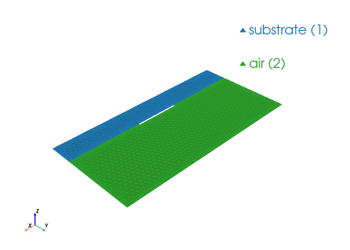
Palace simulation output
Running: /home/runner/.cache/palacetoolkit/runtime/palace-cpu-v0.17.0/bin/palace --serial /tmp/wg_microstrip_h533ge12_modes/config.json
>> /home/runner/.cache/palacetoolkit/runtime/palace-cpu-v0.17.0/bin/palace-x86_64.bin /tmp/wg_microstrip_h533ge12_modes/config.json
_____________ _______
_____ __ \____ __ /____ ____________
____ /_/ / __ ` / / __ ` / ___/ _ \
___ _____/ /_/ / / /_/ / /__/ ___/
/__/ \___,__/__/\___,__/\_____\_____/
Git changeset ID: v0.17.0-272-gb22f654ab
Running with 1 MPI process, 1 OpenMP thread
Device configuration: omp,cpu
Memory configuration: host-std
libCEED backend: /cpu/self/xsmm/blocked
[38;2;255;255;000m--> Warning![0m
One or more external boundary attributes has no associated boundary condition!
"PMC"/"ZeroCharge" condition is assumed!
Boundary attribute list: 3
Characteristic length and time scales:
Lc = 8.000e+00 m, tc = 2.669e+01 ns
Finished partitioning mesh into 1 subdomain
Mesh curvature order: 1
Mesh bounding box:
(Xmin, Ymin) = (-4.000e+00, -1.000e+00) m
(Xmax, Ymax) = (+4.000e+00, +3.000e+00) m
Parallel Mesh Stats:
minimum average maximum total
vertices 3156 3156 3156 3156
edges 8934 8934 8934 8934
elements 5778 5778 5778 5778
neighbors 0 0 0
minimum maximum
h 0.00449751 0.0255824
kappa 1 2.60387
Estimated current per-rank memory usage is: Min. 45.8M, Max. 45.8M, Avg. 45.8M, Total 45.8M
Estimated current per-node memory usage is: Min. 45.8M, Max. 45.8M, Avg. 45.8M, Total 45.8M
Configuring 2D waveguide mode analysis at f = 4.775e-02 GHz (omega = 8.005538e+00)
ND space: 29424 DOFs, H1 space: 12090 DOFs, total: 41514
Auto kn_target = 1.839533e+01 (from max(mu_r) * max(epsilon_r) = 4.800000e+00)
Solving GEP for 8 propagation mode(s)...
Residual norms for GMRES solve
0 (restart 0) KSP residual norm 2.590173e-01
1 (restart 0) KSP residual norm 3.481167e-14
GMRES solver converged in 1 iteration (avg. reduction factor: 1.344e-13)
Residual norms for GMRES solve
0 (restart 0) KSP residual norm 4.185439e-02
1 (restart 0) KSP residual norm 5.448553e-15
GMRES solver converged in 1 iteration (avg. reduction factor: 1.302e-13)
Residual norms for GMRES solve
0 (restart 0) KSP residual norm 6.230912e-02
1 (restart 0) KSP residual norm 6.928465e-15
GMRES solver converged in 1 iteration (avg. reduction factor: 1.112e-13)
Residual norms for GMRES solve
0 (restart 0) KSP residual norm 3.704263e-02
1 (restart 0) KSP residual norm 5.932042e-15
GMRES solver converged in 1 iteration (avg. reduction factor: 1.601e-13)
Residual norms for GMRES solve
0 (restart 0) KSP residual norm 1.378110e-02
1 (restart 0) KSP residual norm 2.366519e-15
GMRES solver converged in 1 iteration (avg. reduction factor: 1.717e-13)
Residual norms for GMRES solve
0 (restart 0) KSP residual norm 2.597370e-02
1 (restart 0) KSP residual norm 5.166790e-15
GMRES solver converged in 1 iteration (avg. reduction factor: 1.989e-13)
Residual norms for GMRES solve
0 (restart 0) KSP residual norm 1.755998e-02
1 (restart 0) KSP residual norm 2.826152e-15
GMRES solver converged in 1 iteration (avg. reduction factor: 1.609e-13)
Residual norms for GMRES solve
0 (restart 0) KSP residual norm 2.656758e-02
1 (restart 0) KSP residual norm 3.578343e-15
GMRES solver converged in 1 iteration (avg. reduction factor: 1.347e-13)
Residual norms for GMRES solve
0 (restart 0) KSP residual norm 1.707955e-02
1 (restart 0) KSP residual norm 4.737590e-15
GMRES solver converged in 1 iteration (avg. reduction factor: 2.774e-13)
Residual norms for GMRES solve
0 (restart 0) KSP residual norm 2.201716e-02
1 (restart 0) KSP residual norm 2.783592e-15
GMRES solver converged in 1 iteration (avg. reduction factor: 1.264e-13)
Residual norms for GMRES solve
0 (restart 0) KSP residual norm 2.254559e-02
1 (restart 0) KSP residual norm 3.292945e-15
GMRES solver converged in 1 iteration (avg. reduction factor: 1.461e-13)
Residual norms for GMRES solve
0 (restart 0) KSP residual norm 1.109895e-02
1 (restart 0) KSP residual norm 2.589177e-15
GMRES solver converged in 1 iteration (avg. reduction factor: 2.333e-13)
Residual norms for GMRES solve
0 (restart 0) KSP residual norm 3.579156e-02
1 (restart 0) KSP residual norm 4.230657e-15
GMRES solver converged in 1 iteration (avg. reduction factor: 1.182e-13)
Residual norms for GMRES solve
0 (restart 0) KSP residual norm 1.395744e-02
1 (restart 0) KSP residual norm 2.664015e-15
GMRES solver converged in 1 iteration (avg. reduction factor: 1.909e-13)
Residual norms for GMRES solve
0 (restart 0) KSP residual norm 1.417757e-02
1 (restart 0) KSP residual norm 3.698612e-15
GMRES solver converged in 1 iteration (avg. reduction factor: 2.609e-13)
Residual norms for GMRES solve
0 (restart 0) KSP residual norm 2.736284e-02
1 (restart 0) KSP residual norm 7.303943e-15
GMRES solver converged in 1 iteration (avg. reduction factor: 2.669e-13)
Residual norms for GMRES solve
0 (restart 0) KSP residual norm 2.226306e-02
1 (restart 0) KSP residual norm 6.227593e-15
GMRES solver converged in 1 iteration (avg. reduction factor: 2.797e-13)
Residual norms for GMRES solve
0 (restart 0) KSP residual norm 1.941762e-02
1 (restart 0) KSP residual norm 2.898725e-15
GMRES solver converged in 1 iteration (avg. reduction factor: 1.493e-13)
Residual norms for GMRES solve
0 (restart 0) KSP residual norm 4.319402e-02
1 (restart 0) KSP residual norm 7.721818e-15
GMRES solver converged in 1 iteration (avg. reduction factor: 1.788e-13)
Residual norms for GMRES solve
0 (restart 0) KSP residual norm 5.056058e-02
1 (restart 0) KSP residual norm 8.049420e-15
GMRES solver converged in 1 iteration (avg. reduction factor: 1.592e-13)
Residual norms for GMRES solve
0 (restart 0) KSP residual norm 1.522852e-02
1 (restart 0) KSP residual norm 6.054436e-15
GMRES solver converged in 1 iteration (avg. reduction factor: 3.976e-13)
Residual norms for GMRES solve
0 (restart 0) KSP residual norm 1.004315e-02
1 (restart 0) KSP residual norm 6.238537e-15
GMRES solver converged in 1 iteration (avg. reduction factor: 6.212e-13)
Residual norms for GMRES solve
0 (restart 0) KSP residual norm 9.249603e-03
1 (restart 0) KSP residual norm 2.696847e-15
GMRES solver converged in 1 iteration (avg. reduction factor: 2.916e-13)
Residual norms for GMRES solve
0 (restart 0) KSP residual norm 9.298013e-03
1 (restart 0) KSP residual norm 4.502345e-15
GMRES solver converged in 1 iteration (avg. reduction factor: 4.842e-13)
Residual norms for GMRES solve
0 (restart 0) KSP residual norm 1.586526e-02
1 (restart 0) KSP residual norm 5.450039e-15
GMRES solver converged in 1 iteration (avg. reduction factor: 3.435e-13)
Residual norms for GMRES solve
0 (restart 0) KSP residual norm 8.059502e-03
1 (restart 0) KSP residual norm 3.840585e-15
GMRES solver converged in 1 iteration (avg. reduction factor: 4.765e-13)
Residual norms for GMRES solve
0 (restart 0) KSP residual norm 2.006125e-02
1 (restart 0) KSP residual norm 5.800473e-15
GMRES solver converged in 1 iteration (avg. reduction factor: 2.891e-13)
Residual norms for GMRES solve
0 (restart 0) KSP residual norm 1.579398e-02
1 (restart 0) KSP residual norm 6.931195e-15
GMRES solver converged in 1 iteration (avg. reduction factor: 4.389e-13)
Residual norms for GMRES solve
0 (restart 0) KSP residual norm 9.190050e-03
1 (restart 0) KSP residual norm 3.791329e-15
GMRES solver converged in 1 iteration (avg. reduction factor: 4.125e-13)
Residual norms for GMRES solve
0 (restart 0) KSP residual norm 1.066442e-02
1 (restart 0) KSP residual norm 5.592713e-15
GMRES solver converged in 1 iteration (avg. reduction factor: 5.244e-13)
Residual norms for GMRES solve
0 (restart 0) KSP residual norm 1.436135e-02
1 (restart 0) KSP residual norm 9.533966e-15
GMRES solver converged in 1 iteration (avg. reduction factor: 6.639e-13)
Residual norms for GMRES solve
0 (restart 0) KSP residual norm 8.989860e-03
1 (restart 0) KSP residual norm 7.071390e-15
GMRES solver converged in 1 iteration (avg. reduction factor: 7.866e-13)
Residual norms for GMRES solve
0 (restart 0) KSP residual norm 7.313331e-03
1 (restart 0) KSP residual norm 5.937417e-15
GMRES solver converged in 1 iteration (avg. reduction factor: 8.119e-13)
Residual norms for GMRES solve
0 (restart 0) KSP residual norm 6.874409e-03
1 (restart 0) KSP residual norm 1.013116e-14
GMRES solver converged in 1 iteration (avg. reduction factor: 1.474e-12)
Residual norms for GMRES solve
0 (restart 0) KSP residual norm 6.068884e-03
1 (restart 0) KSP residual norm 1.773735e-14
GMRES solver converged in 1 iteration (avg. reduction factor: 2.923e-12)
Residual norms for GMRES solve
0 (restart 0) KSP residual norm 1.587518e-02
1 (restart 0) KSP residual norm 2.637572e-14
GMRES solver converged in 1 iteration (avg. reduction factor: 1.661e-12)
Residual norms for GMRES solve
0 (restart 0) KSP residual norm 9.266762e-03
1 (restart 0) KSP residual norm 1.294532e-14
GMRES solver converged in 1 iteration (avg. reduction factor: 1.397e-12)
Residual norms for GMRES solve
0 (restart 0) KSP residual norm 1.226467e-02
1 (restart 0) KSP residual norm 1.058781e-14
GMRES solver converged in 1 iteration (avg. reduction factor: 8.633e-13)
Residual norms for GMRES solve
0 (restart 0) KSP residual norm 1.664414e-02
1 (restart 0) KSP residual norm 1.544782e-14
GMRES solver converged in 1 iteration (avg. reduction factor: 9.281e-13)
Residual norms for GMRES solve
0 (restart 0) KSP residual norm 1.501050e-02
1 (restart 0) KSP residual norm 2.251733e-14
GMRES solver converged in 1 iteration (avg. reduction factor: 1.500e-12)
Residual norms for GMRES solve
0 (restart 0) KSP residual norm 2.590403e-02
1 (restart 0) KSP residual norm 4.321432e-14
GMRES solver converged in 1 iteration (avg. reduction factor: 1.668e-12)
Residual norms for GMRES solve
0 (restart 0) KSP residual norm 1.817729e-02
1 (restart 0) KSP residual norm 4.223855e-14
GMRES solver converged in 1 iteration (avg. reduction factor: 2.324e-12)
Residual norms for GMRES solve
0 (restart 0) KSP residual norm 3.241467e-02
1 (restart 0) KSP residual norm 4.968137e-14
GMRES solver converged in 1 iteration (avg. reduction factor: 1.533e-12)
Residual norms for GMRES solve
0 (restart 0) KSP residual norm 1.920000e-02
1 (restart 0) KSP residual norm 3.137853e-14
GMRES solver converged in 1 iteration (avg. reduction factor: 1.634e-12)
Residual norms for GMRES solve
0 (restart 0) KSP residual norm 2.267319e-02
1 (restart 0) KSP residual norm 3.435030e-14
GMRES solver converged in 1 iteration (avg. reduction factor: 1.515e-12)
Residual norms for GMRES solve
0 (restart 0) KSP residual norm 1.673746e-02
1 (restart 0) KSP residual norm 3.264096e-14
GMRES solver converged in 1 iteration (avg. reduction factor: 1.950e-12)
Residual norms for GMRES solve
0 (restart 0) KSP residual norm 1.783290e-02
1 (restart 0) KSP residual norm 3.468781e-14
GMRES solver converged in 1 iteration (avg. reduction factor: 1.945e-12)
Residual norms for GMRES solve
0 (restart 0) KSP residual norm 1.809951e-02
1 (restart 0) KSP residual norm 3.218267e-14
GMRES solver converged in 1 iteration (avg. reduction factor: 1.778e-12)
Residual norms for GMRES solve
0 (restart 0) KSP residual norm 1.074876e-02
1 (restart 0) KSP residual norm 1.199238e-14
GMRES solver converged in 1 iteration (avg. reduction factor: 1.116e-12)
Residual norms for GMRES solve
0 (restart 0) KSP residual norm 1.984934e-02
1 (restart 0) KSP residual norm 1.626256e-14
GMRES solver converged in 1 iteration (avg. reduction factor: 8.193e-13)
Residual norms for GMRES solve
0 (restart 0) KSP residual norm 1.542955e-02
1 (restart 0) KSP residual norm 2.362645e-14
GMRES solver converged in 1 iteration (avg. reduction factor: 1.531e-12)
Residual norms for GMRES solve
0 (restart 0) KSP residual norm 1.148409e-02
1 (restart 0) KSP residual norm 2.057029e-14
GMRES solver converged in 1 iteration (avg. reduction factor: 1.791e-12)
Residual norms for GMRES solve
0 (restart 0) KSP residual norm 1.440093e-02
1 (restart 0) KSP residual norm 2.491651e-14
GMRES solver converged in 1 iteration (avg. reduction factor: 1.730e-12)
Residual norms for GMRES solve
0 (restart 0) KSP residual norm 1.567960e-02
1 (restart 0) KSP residual norm 2.887297e-14
GMRES solver converged in 1 iteration (avg. reduction factor: 1.841e-12)
Residual norms for GMRES solve
0 (restart 0) KSP residual norm 1.962330e-02
1 (restart 0) KSP residual norm 1.754161e-14
GMRES solver converged in 1 iteration (avg. reduction factor: 8.939e-13)
Residual norms for GMRES solve
0 (restart 0) KSP residual norm 1.450862e-02
1 (restart 0) KSP residual norm 1.388439e-14
GMRES solver converged in 1 iteration (avg. reduction factor: 9.570e-13)
Residual norms for GMRES solve
0 (restart 0) KSP residual norm 1.792107e-02
1 (restart 0) KSP residual norm 2.135657e-14
GMRES solver converged in 1 iteration (avg. reduction factor: 1.192e-12)
Residual norms for GMRES solve
0 (restart 0) KSP residual norm 1.341649e-02
1 (restart 0) KSP residual norm 2.312616e-14
GMRES solver converged in 1 iteration (avg. reduction factor: 1.724e-12)
Residual norms for GMRES solve
0 (restart 0) KSP residual norm 1.450146e-02
1 (restart 0) KSP residual norm 2.496273e-14
GMRES solver converged in 1 iteration (avg. reduction factor: 1.721e-12)
Residual norms for GMRES solve
0 (restart 0) KSP residual norm 1.666416e-02
1 (restart 0) KSP residual norm 3.156932e-14
GMRES solver converged in 1 iteration (avg. reduction factor: 1.894e-12)
Found 11 converged eigenvalues (sigma = -3.383880e+02)
eig 0: kn = 1.678566e+01-5.553056e-15i, n_eff = 2.096756e+00-6.936518e-16i
eig 1: kn = 1.406124e+01-1.081990e-11i, n_eff = 1.756439e+00-1.351552e-12i
eig 2: kn = 1.302446e+01-8.638570e-10i, n_eff = 1.626931e+00-1.079074e-10i
eig 3: kn = 1.225619e+01+8.960040e-08i, n_eff = 1.530964e+00+1.119230e-08i
eig 4: kn = 8.941567e+00+1.006723e-09i, n_eff = 1.116923e+00+1.257533e-10i
eig 5: kn = 8.557204e+00+1.068240e-07i, n_eff = 1.068911e+00+1.334376e-08i
eig 6: kn = 6.883905e+00+4.994699e-10i, n_eff = 8.598929e-01+6.239055e-11i
eig 7: kn = 5.399019e+00+3.001458e-09i, n_eff = 6.744105e-01+3.749227e-10i
eig 8: kn = 5.375352e+00+1.003187e-07i, n_eff = 6.714542e-01+1.253116e-08i
eig 9: kn = 4.115671e+00+1.226945e-07i, n_eff = 5.141029e-01+1.532621e-08i
eig 10: kn = 2.175968e+00-4.514641e-08i, n_eff = 2.718078e-01-5.639397e-09i
Computing solution error estimates and performing postprocessing
m, Re{kn} (1/m), Im{kn} (1/m), Re{n_eff}, Im{n_eff}, Error (Bkwd.), Error (Abs.)
1, +2.098207e+00, -6.941320e-16, +2.096756e+00, -6.936518e-16, +1.440906e-16, +1.857176e-12
2, +1.757655e+00, -1.352487e-12, +1.756439e+00, -1.351552e-12, +2.008180e-15, +1.042161e-11
3, +1.628057e+00, -1.079821e-10, +1.626931e+00, -1.079074e-10, +2.464006e-13, +1.065983e-09
4, +1.532024e+00, +1.120005e-08, +1.530964e+00, +1.119230e-08, +6.572234e-12, +2.549918e-08
5, +1.117696e+00, +1.258404e-10, +1.116923e+00, +1.257533e-10, +1.156687e-13, +3.268088e-10
6, +1.069651e+00, +1.335300e-08, +1.068911e+00, +1.334376e-08, +5.743716e-12, +1.581679e-08
7, +8.604882e-01, +6.243374e-11, +8.598929e-01, +6.239055e-11, +4.584339e-13, +1.150384e-09
8, +6.748773e-01, +3.751822e-10, +6.744105e-01, +3.749227e-10, +3.161904e-13, +7.466707e-10
Completed 0 iterations of adaptive mesh refinement (AMR):
Indicator norm = 2.602e-02, global unknowns = 41514
Max. iterations = 0, tol. = 1.000e-02
Estimated peak per-rank memory usage is: Min. 286.6M, Max. 286.6M, Avg. 286.6M, Total 286.6M
Estimated peak per-node memory usage is: Min. 286.6M, Max. 286.6M, Avg. 286.6M, Total 286.6M
Elapsed Time Report (s) Min. Max. Avg.
==============================================================
Initialization 0.013 0.013 0.013
Mesh Preprocessing 0.036 0.036 0.036
Operator Construction 0.092 0.092 0.092
Preconditioner 1.887 1.887 1.887
Eigenvalue Solve 0.398 0.398 0.398
Estimation 0.033 0.033 0.033
Construction 0.190 0.190 0.190
Solve 0.648 0.648 0.648
Postprocessing 2.053 2.053 2.053
Disk IO 0.011 0.011 0.011
--------------------------------------------------------------
Total 5.636 5.636 5.636
Peak Memory Per-Node Total Total HWM
==============================================================
Initialization 2.0M 2.0M 2.0M
Mesh Preprocessing 3.4M 3.4M 5.3M
Operator Construction 44.1M 44.1M 49.4M
Preconditioner 128.9M 128.9M 178.3M
Eigenvalue Solve 54.3M 54.3M 232.7M
Estimation 0.0K 0.0K 232.7M
Construction 13.6M 13.6M 246.3M
Solve 0.0K 0.0K 246.3M
Postprocessing 0.0K 0.0K 246.3M
Disk IO 2.5M 2.5M 248.8M
--------------------------------------------------------------
Total 261.4M 261.4M 261.4MComputed microstrip modes:
Mode 1: kn= +2.098207 -0.000000j [bound/hybrid]
# Field visualization is no longer available through the solver.
# Palace writes VTU field output files when save > 0 in solver.solve().
# Load the VTU files with pyvista for field visualization.
# For more details, see palacetoolkit.postpro_vtu utilities.
print("Field visualization moved to pyvista-based VTU post-processing.")
Field visualization moved to pyvista-based VTU post-processing.
Validation vs. Hammerstad-Jensen#
To validate loss prediction, we compare transmission magnitude estimated from solver-derived effective permittivity against a Hammerstad-Jensen-based dielectric-loss model.
Validation sweep setup (kept comfortably inside commonly used validity limits):
Relative permittivity: \(2.2 \le \varepsilon_r \le 6.15\)
Width ratio: \(0.8 \le w/h \le 2.5\)
Thin strip: \(t/h = 0.04\)
Low-loss dielectric: \(\tan\delta = 0.002\)
For each case, we compute:
Solver-derived: run eigenmode with real \(\varepsilon_r\), infer \(\varepsilon_{\mathrm{eff,solver}}=(\Re\{k_n\}/\omega)^2/\mu_r\), then use low-loss dielectric estimate for \(\alpha\)
HJ-based reference: \(|S_{21}|_{\mathrm{HJ}} \approx e^{-\alpha_{\mathrm{HJ}}L}\) using \(\varepsilon_{\mathrm{eff,HJ}}\) and a quasi-static dielectric filling factor
Impedance comparison: two numerical estimates are used: (i) contour-based \(Z_{0,VI}=|V/I|\) and (ii) quasi-static energy/capacitance estimate \(Z_{0,C}\), both compared to analytic \(Z_{0,\mathrm{HJ}}\)
Low-loss approximation used in this cell:
For a weakly lossy dielectric, write the propagation constant as \(\gamma = \alpha + j\beta\) and use \(\varepsilon = \varepsilon'(1-j\tan\delta_{\mathrm{eff}})\) with \(\tan\delta_{\mathrm{eff}} \ll 1\).
First-order expansion gives \(\alpha \approx \tfrac{\beta}{2}\tan\delta_{\mathrm{eff}}\).
In quasi-TEM form, \(\beta \approx \omega\sqrt{\mu_r\varepsilon_{\mathrm{eff}}}\).
We estimate \(\tan\delta_{\mathrm{eff}} = q\,\tan\delta\) with filling factor \(q \approx (\varepsilon_{\mathrm{eff}}-1)/(\varepsilon_r-1)\).
Therefore, \(\alpha \approx \tfrac{1}{2}\,\omega\sqrt{\mu_r\varepsilon_{\mathrm{eff}}}\,q\tan\delta\) and \(|S_{21}| \approx e^{-\alpha L}\).
Note: this eigenmode setup uses PEC conductors and real-valued material tensors, so this section validates dielectric loss contribution (not conductor loss).
def hammerstad_jensen_eps_eff(er, u):
    if u <= 0:
        raise ValueError("u = w/h must be positive")
    a = 1.0 + (1.0 / 49.0) * np.log((u**4 + (u / 52.0) ** 2) / (u**4 + 0.432))
    a += (1.0 / 18.7) * np.log(1.0 + u / 18.1)
    b = 0.564 * ((er - 0.9) / (er + 3.0)) ** 0.053
    return 0.5 * (er + 1.0) + 0.5 * (er - 1.0) * (1.0 + 10.0 / u) ** (-a * b)


def hj_dielectric_alpha(omega, er, eeff, tand):
    q = (eeff - 1.0) / max(er - 1.0, 1e-12)
    tand_eff = q * tand
    beta_hj = omega * np.sqrt(mu_r * eeff)
    return 0.5 * beta_hj * tand_eff


def hammerstad_jensen_z0(er, u):
    eeff = hammerstad_jensen_eps_eff(er, u)
    f = 6.0 + (2.0 * np.pi - 6.0) * np.exp(-((30.666 / u) ** 0.7528))
    return (60.0 / np.sqrt(eeff)) * np.log(f / u + np.sqrt(1.0 + (2.0 / u) ** 2))


def pick_guided_mode(kn_vals, omega, mu_r, eps_air, eps_sub):
    k_air = omega * np.sqrt(mu_r * eps_air)
    k_sub = omega * np.sqrt(mu_r * eps_sub)
    guided = [
        kn for kn in kn_vals
        if (k_air * 1.001) < kn.real < (k_sub * 0.999) and abs(kn.imag) < 0.05 * max(abs(kn.real), 1e-12)
    ]
    if guided:
        return sorted(guided, key=lambda z: z.real)[-1]
    return sorted(kn_vals, key=lambda z: abs(z.imag))[0]


validation_cases = [
    {"eps_sub": 2.2, "w_over_h": 0.8},
    {"eps_sub": 2.2, "w_over_h": 1.6},
    {"eps_sub": 4.4, "w_over_h": 1.0},
    {"eps_sub": 4.4, "w_over_h": 2.0},
    {"eps_sub": 6.15, "w_over_h": 1.2},
    {"eps_sub": 6.15, "w_over_h": 2.5},
]

h_sub_val = 1.0
h_air_val = 3.0
box_w_val = 8.0
strip_t_val = 0.04 * h_sub_val
tand_sub = 0.002
line_length = 40.0 * h_sub_val
eta0 = 376.730313668
meshsize_val = 1.0

rows = []
for case in validation_cases:
    er = case["eps_sub"]
    u = case["w_over_h"]
    strip_w = u * h_sub_val

    mesh_case = make_microstrip_mesh(
        box_w=box_w_val,
        h_sub=h_sub_val,
        h_air=h_air_val,
        strip_w=strip_w,
        strip_t=strip_t_val,
        lc_bulk=0.18,
        lc_strip=0.05,
        meshsize=meshsize_val,
    )

    solver_case = WaveguideModeSolver(
        mesh_file=mesh_case,
        order=2,
        pec_bdr=pec_bdr,
        materials=[
            {"attrs": [1], "eps_r": er, "mu_r": mu_r},
            {"attrs": [2], "eps_r": eps_air, "mu_r": mu_r},
        ],
        omega=omega,
    )
    res_case = solver_case.solve(num_modes=8, mode_idx=1, target=0.0, save=0, num_procs=4)

    kn_vals = [res_case[i].k_n for i in sorted(res_case)]
    kn_pick = pick_guided_mode(kn_vals, omega, mu_r, eps_air, er)
    eps_eff_solver = (kn_pick.real / omega) ** 2 / mu_r
    alpha_solver = hj_dielectric_alpha(omega, er, eps_eff_solver, tand_sub)
    s21_solver = np.exp(-alpha_solver * line_length)

    eps_eff_hj = hammerstad_jensen_eps_eff(er, u)
    alpha_hj = hj_dielectric_alpha(omega, er, eps_eff_hj, tand_sub)
    s21_hj = np.exp(-alpha_hj * line_length)
    z0_hj = hammerstad_jensen_z0(er, u)

    eps_eff_err_pct = 100.0 * (eps_eff_solver - eps_eff_hj) / max(eps_eff_hj, 1e-12)
    err_pct = 100.0 * (s21_solver - s21_hj) / max(s21_hj, 1e-12)
    il_solver_db = -20.0 * np.log10(max(s21_solver, 1e-14))
    il_hj_db = -20.0 * np.log10(max(s21_hj, 1e-14))
    rows.append((er, u, eps_eff_solver, eps_eff_hj, eps_eff_err_pct, s21_solver, s21_hj, err_pct, z0_hj, il_solver_db, il_hj_db))
Palace simulation output
Running: /home/runner/.cache/palacetoolkit/runtime/palace-cpu-v0.17.0/bin/palace --serial /tmp/wg_microstrip_86haqtjg_modes/config.json
>> /home/runner/.cache/palacetoolkit/runtime/palace-cpu-v0.17.0/bin/palace-x86_64.bin /tmp/wg_microstrip_86haqtjg_modes/config.json
_____________ _______
_____ __ \____ __ /____ ____________
____ /_/ / __ ` / / __ ` / ___/ _ \
___ _____/ /_/ / / /_/ / /__/ ___/
/__/ \___,__/__/\___,__/\_____\_____/
Git changeset ID: v0.17.0-272-gb22f654ab
Running with 1 MPI process, 1 OpenMP thread
Device configuration: omp,cpu
Memory configuration: host-std
libCEED backend: /cpu/self/xsmm/blocked
[38;2;255;255;000m--> Warning![0m
One or more external boundary attributes has no associated boundary condition!
"PMC"/"ZeroCharge" condition is assumed!
Boundary attribute list: 3
Characteristic length and time scales:
Lc = 8.000e+00 m, tc = 2.669e+01 ns
Finished partitioning mesh into 1 subdomain
Mesh curvature order: 1
Mesh bounding box:
(Xmin, Ymin) = (-4.000e+00, -1.000e+00) m
(Xmax, Ymax) = (+4.000e+00, +3.000e+00) m
Parallel Mesh Stats:
minimum average maximum total
vertices 3155 3155 3155 3155
edges 8973 8973 8973 8973
elements 5818 5818 5818 5818
neighbors 0 0 0
minimum maximum
h 0.00467942 0.0262638
kappa 1 2.49462
Estimated current per-rank memory usage is: Min. 45.9M, Max. 45.9M, Avg. 45.9M, Total 45.9M
Estimated current per-node memory usage is: Min. 45.9M, Max. 45.9M, Avg. 45.9M, Total 45.9M
Configuring 2D waveguide mode analysis at f = 4.775e-02 GHz (omega = 8.005538e+00)
ND space: 29582 DOFs, H1 space: 12128 DOFs, total: 41710
Auto kn_target = 1.245369e+01 (from max(mu_r) * max(epsilon_r) = 2.200000e+00)
Solving GEP for 8 propagation mode(s)...
Residual norms for GMRES solve
0 (restart 0) KSP residual norm 3.100965e-01
1 (restart 0) KSP residual norm 2.449311e-13
GMRES solver converged in 1 iteration (avg. reduction factor: 7.899e-13)
Residual norms for GMRES solve
0 (restart 0) KSP residual norm 7.133806e-02
1 (restart 0) KSP residual norm 5.632323e-14
GMRES solver converged in 1 iteration (avg. reduction factor: 7.895e-13)
Residual norms for GMRES solve
0 (restart 0) KSP residual norm 3.330713e-02
1 (restart 0) KSP residual norm 2.982455e-14
GMRES solver converged in 1 iteration (avg. reduction factor: 8.954e-13)
Residual norms for GMRES solve
0 (restart 0) KSP residual norm 9.183260e-02
1 (restart 0) KSP residual norm 7.508114e-14
GMRES solver converged in 1 iteration (avg. reduction factor: 8.176e-13)
Residual norms for GMRES solve
0 (restart 0) KSP residual norm 6.034076e-02
1 (restart 0) KSP residual norm 4.327685e-14
GMRES solver converged in 1 iteration (avg. reduction factor: 7.172e-13)
Residual norms for GMRES solve
0 (restart 0) KSP residual norm 3.039053e-02
1 (restart 0) KSP residual norm 2.628215e-14
GMRES solver converged in 1 iteration (avg. reduction factor: 8.648e-13)
Residual norms for GMRES solve
0 (restart 0) KSP residual norm 3.091490e-02
1 (restart 0) KSP residual norm 2.006775e-14
GMRES solver converged in 1 iteration (avg. reduction factor: 6.491e-13)
Residual norms for GMRES solve
0 (restart 0) KSP residual norm 3.127585e-02
1 (restart 0) KSP residual norm 2.776407e-14
GMRES solver converged in 1 iteration (avg. reduction factor: 8.877e-13)
Residual norms for GMRES solve
0 (restart 0) KSP residual norm 3.924276e-02
1 (restart 0) KSP residual norm 4.317134e-14
GMRES solver converged in 1 iteration (avg. reduction factor: 1.100e-12)
Residual norms for GMRES solve
0 (restart 0) KSP residual norm 4.183523e-02
1 (restart 0) KSP residual norm 4.584828e-14
GMRES solver converged in 1 iteration (avg. reduction factor: 1.096e-12)
Residual norms for GMRES solve
0 (restart 0) KSP residual norm 3.493977e-02
1 (restart 0) KSP residual norm 2.443161e-14
GMRES solver converged in 1 iteration (avg. reduction factor: 6.992e-13)
Residual norms for GMRES solve
0 (restart 0) KSP residual norm 5.538677e-02
1 (restart 0) KSP residual norm 4.371561e-14
GMRES solver converged in 1 iteration (avg. reduction factor: 7.893e-13)
Residual norms for GMRES solve
0 (restart 0) KSP residual norm 3.276773e-02
1 (restart 0) KSP residual norm 3.624484e-14
GMRES solver converged in 1 iteration (avg. reduction factor: 1.106e-12)
Residual norms for GMRES solve
0 (restart 0) KSP residual norm 5.181967e-02
1 (restart 0) KSP residual norm 5.986165e-14
GMRES solver converged in 1 iteration (avg. reduction factor: 1.155e-12)
Residual norms for GMRES solve
0 (restart 0) KSP residual norm 1.643933e-02
1 (restart 0) KSP residual norm 1.768413e-14
GMRES solver converged in 1 iteration (avg. reduction factor: 1.076e-12)
Residual norms for GMRES solve
0 (restart 0) KSP residual norm 2.276258e-02
1 (restart 0) KSP residual norm 1.904419e-14
GMRES solver converged in 1 iteration (avg. reduction factor: 8.366e-13)
Residual norms for GMRES solve
0 (restart 0) KSP residual norm 2.974824e-02
1 (restart 0) KSP residual norm 2.894041e-14
GMRES solver converged in 1 iteration (avg. reduction factor: 9.728e-13)
Residual norms for GMRES solve
0 (restart 0) KSP residual norm 5.738354e-02
1 (restart 0) KSP residual norm 4.863350e-14
GMRES solver converged in 1 iteration (avg. reduction factor: 8.475e-13)
Residual norms for GMRES solve
0 (restart 0) KSP residual norm 4.145720e-02
1 (restart 0) KSP residual norm 4.360416e-14
GMRES solver converged in 1 iteration (avg. reduction factor: 1.052e-12)
Residual norms for GMRES solve
0 (restart 0) KSP residual norm 2.039118e-02
1 (restart 0) KSP residual norm 6.589813e-14
GMRES solver converged in 1 iteration (avg. reduction factor: 3.232e-12)
Residual norms for GMRES solve
0 (restart 0) KSP residual norm 2.535613e-02
1 (restart 0) KSP residual norm 7.866970e-14
GMRES solver converged in 1 iteration (avg. reduction factor: 3.103e-12)
Residual norms for GMRES solve
0 (restart 0) KSP residual norm 1.705886e-02
1 (restart 0) KSP residual norm 5.613727e-14
GMRES solver converged in 1 iteration (avg. reduction factor: 3.291e-12)
Residual norms for GMRES solve
0 (restart 0) KSP residual norm 2.354642e-02
1 (restart 0) KSP residual norm 9.039674e-14
GMRES solver converged in 1 iteration (avg. reduction factor: 3.839e-12)
Residual norms for GMRES solve
0 (restart 0) KSP residual norm 3.288240e-02
1 (restart 0) KSP residual norm 1.771054e-13
GMRES solver converged in 1 iteration (avg. reduction factor: 5.386e-12)
Residual norms for GMRES solve
0 (restart 0) KSP residual norm 2.953435e-02
1 (restart 0) KSP residual norm 5.932635e-14
GMRES solver converged in 1 iteration (avg. reduction factor: 2.009e-12)
Residual norms for GMRES solve
0 (restart 0) KSP residual norm 3.056241e-02
1 (restart 0) KSP residual norm 7.922502e-14
GMRES solver converged in 1 iteration (avg. reduction factor: 2.592e-12)
Residual norms for GMRES solve
0 (restart 0) KSP residual norm 2.912015e-02
1 (restart 0) KSP residual norm 3.164044e-14
GMRES solver converged in 1 iteration (avg. reduction factor: 1.087e-12)
Residual norms for GMRES solve
0 (restart 0) KSP residual norm 7.635564e-02
1 (restart 0) KSP residual norm 8.523420e-14
GMRES solver converged in 1 iteration (avg. reduction factor: 1.116e-12)
Residual norms for GMRES solve
0 (restart 0) KSP residual norm 1.647252e-02
1 (restart 0) KSP residual norm 4.486647e-14
GMRES solver converged in 1 iteration (avg. reduction factor: 2.724e-12)
Residual norms for GMRES solve
0 (restart 0) KSP residual norm 4.056225e-02
1 (restart 0) KSP residual norm 3.869649e-14
GMRES solver converged in 1 iteration (avg. reduction factor: 9.540e-13)
Residual norms for GMRES solve
0 (restart 0) KSP residual norm 4.873419e-02
1 (restart 0) KSP residual norm 4.414710e-14
GMRES solver converged in 1 iteration (avg. reduction factor: 9.059e-13)
Residual norms for GMRES solve
0 (restart 0) KSP residual norm 5.457925e-02
1 (restart 0) KSP residual norm 7.884669e-14
GMRES solver converged in 1 iteration (avg. reduction factor: 1.445e-12)
Residual norms for GMRES solve
0 (restart 0) KSP residual norm 2.969016e-02
1 (restart 0) KSP residual norm 6.356812e-14
GMRES solver converged in 1 iteration (avg. reduction factor: 2.141e-12)
Residual norms for GMRES solve
0 (restart 0) KSP residual norm 3.068665e-02
1 (restart 0) KSP residual norm 7.125392e-14
GMRES solver converged in 1 iteration (avg. reduction factor: 2.322e-12)
Residual norms for GMRES solve
0 (restart 0) KSP residual norm 3.598087e-02
1 (restart 0) KSP residual norm 6.294157e-14
GMRES solver converged in 1 iteration (avg. reduction factor: 1.749e-12)
Residual norms for GMRES solve
0 (restart 0) KSP residual norm 2.747376e-02
1 (restart 0) KSP residual norm 6.629319e-14
GMRES solver converged in 1 iteration (avg. reduction factor: 2.413e-12)
Residual norms for GMRES solve
0 (restart 0) KSP residual norm 3.602932e-02
1 (restart 0) KSP residual norm 5.470250e-14
GMRES solver converged in 1 iteration (avg. reduction factor: 1.518e-12)
Residual norms for GMRES solve
0 (restart 0) KSP residual norm 2.723347e-02
1 (restart 0) KSP residual norm 3.762057e-14
GMRES solver converged in 1 iteration (avg. reduction factor: 1.381e-12)
Residual norms for GMRES solve
0 (restart 0) KSP residual norm 1.875013e-02
1 (restart 0) KSP residual norm 3.187179e-14
GMRES solver converged in 1 iteration (avg. reduction factor: 1.700e-12)
Residual norms for GMRES solve
0 (restart 0) KSP residual norm 2.610296e-02
1 (restart 0) KSP residual norm 2.536810e-14
GMRES solver converged in 1 iteration (avg. reduction factor: 9.718e-13)
Residual norms for GMRES solve
0 (restart 0) KSP residual norm 4.060724e-02
1 (restart 0) KSP residual norm 4.841971e-14
GMRES solver converged in 1 iteration (avg. reduction factor: 1.192e-12)
Residual norms for GMRES solve
0 (restart 0) KSP residual norm 3.149824e-02
1 (restart 0) KSP residual norm 3.295788e-14
GMRES solver converged in 1 iteration (avg. reduction factor: 1.046e-12)
Found 8 converged eigenvalues (sigma = -1.550945e+02)
eig 0: kn = 1.107937e+01-3.823714e-13i, n_eff = 1.383963e+00-4.776336e-14i
eig 1: kn = 8.622523e+00-1.120489e-10i, n_eff = 1.077070e+00-1.399643e-11i
eig 2: kn = 8.531264e+00+1.052084e-11i, n_eff = 1.065670e+00+1.314195e-12i
eig 3: kn = 6.904515e+00+1.734011e-10i, n_eff = 8.624674e-01+2.166014e-11i
eig 4: kn = 6.171195e+00+1.190283e-10i, n_eff = 7.708657e-01+1.486824e-11i
eig 5: kn = 3.711548e+00+3.532015e-08i, n_eff = 4.636226e-01+4.411965e-09i
eig 6: kn = 5.632047e-01-3.827540e-10i, n_eff = 7.035188e-02-4.781115e-11i
eig 7: kn = 1.180189e-07+3.522642e+00i, n_eff = 1.474215e-08+4.400256e-01i
Computing solution error estimates and performing postprocessing
m, Re{kn} (1/m), Im{kn} (1/m), Re{n_eff}, Im{n_eff}, Error (Bkwd.), Error (Abs.)
1, +1.384921e+00, -4.779643e-14, +1.383963e+00, -4.776336e-14, +8.450085e-17, +1.931464e-12
2, +1.077815e+00, -1.400612e-11, +1.077070e+00, -1.399643e-11, +3.921413e-14, +3.590467e-10
3, +1.066408e+00, +1.315105e-12, +1.065670e+00, +1.314195e-12, +1.141299e-13, +1.025109e-09
4, +8.630644e-01, +2.167514e-11, +8.624674e-01, +2.166014e-11, +4.329593e-14, +2.979936e-10
5, +7.713994e-01, +1.487853e-11, +7.708657e-01, +1.486824e-11, +1.042515e-13, +6.587452e-10
6, +4.639435e-01, +4.415019e-09, +4.636226e-01, +4.411965e-09, +6.470439e-13, +3.385431e-09
7, +7.040058e-02, -4.784425e-11, +7.035188e-02, -4.781115e-11, +8.515185e-14, +4.067971e-10
8, +1.475236e-08, +4.403302e-01, +1.474215e-08, +4.400256e-01, +1.808407e-12, +7.983135e-09
Completed 0 iterations of adaptive mesh refinement (AMR):
Indicator norm = 2.223e-02, global unknowns = 41710
Max. iterations = 0, tol. = 1.000e-02
Estimated peak per-rank memory usage is: Min. 296.5M, Max. 296.5M, Avg. 296.5M, Total 296.5M
Estimated peak per-node memory usage is: Min. 296.5M, Max. 296.5M, Avg. 296.5M, Total 296.5M
Elapsed Time Report (s) Min. Max. Avg.
==============================================================
Initialization 0.013 0.013 0.013
Mesh Preprocessing 0.036 0.036 0.036
Operator Construction 0.090 0.090 0.090
Preconditioner 1.409 1.409 1.409
Eigenvalue Solve 0.294 0.294 0.294
Estimation 0.028 0.028 0.028
Construction 0.232 0.232 0.232
Solve 0.583 0.583 0.583
Postprocessing 2.023 2.023 2.023
Disk IO 0.011 0.011 0.011
--------------------------------------------------------------
Total 4.990 4.990 4.990
Peak Memory Per-Node Total Total HWM
==============================================================
Initialization 2.0M 2.0M 2.0M
Mesh Preprocessing 3.3M 3.3M 5.2M
Operator Construction 44.0M 44.0M 49.3M
Preconditioner 138.3M 138.3M 187.5M
Eigenvalue Solve 54.6M 54.6M 242.2M
Estimation 0.0K 0.0K 242.2M
Construction 13.9M 13.9M 256.0M
Solve 0.0K 0.0K 256.0M
Postprocessing 0.0K 0.0K 256.0M
Disk IO 2.5M 2.5M 258.5M
--------------------------------------------------------------
Total 271.2M 271.2M 271.2MPalace simulation output
Running: /home/runner/.cache/palacetoolkit/runtime/palace-cpu-v0.17.0/bin/palace --serial /tmp/wg_microstrip_omx2yuoj_modes/config.json
>> /home/runner/.cache/palacetoolkit/runtime/palace-cpu-v0.17.0/bin/palace-x86_64.bin /tmp/wg_microstrip_omx2yuoj_modes/config.json
_____________ _______
_____ __ \____ __ /____ ____________
____ /_/ / __ ` / / __ ` / ___/ _ \
___ _____/ /_/ / / /_/ / /__/ ___/
/__/ \___,__/__/\___,__/\_____\_____/
Git changeset ID: v0.17.0-272-gb22f654ab
Running with 1 MPI process, 1 OpenMP thread
Device configuration: omp,cpu
Memory configuration: host-std
libCEED backend: /cpu/self/xsmm/blocked
[38;2;255;255;000m--> Warning![0m
One or more external boundary attributes has no associated boundary condition!
"PMC"/"ZeroCharge" condition is assumed!
Boundary attribute list: 3
Characteristic length and time scales:
Lc = 8.000e+00 m, tc = 2.669e+01 ns
Finished partitioning mesh into 1 subdomain
Mesh curvature order: 1
Mesh bounding box:
(Xmin, Ymin) = (-4.000e+00, -1.000e+00) m
(Xmax, Ymax) = (+4.000e+00, +3.000e+00) m
Parallel Mesh Stats:
minimum average maximum total
vertices 3157 3157 3157 3157
edges 8947 8947 8947 8947
elements 5790 5790 5790 5790
neighbors 0 0 0
minimum maximum
h 0.00466725 0.0261352
kappa 1 2.95169
Estimated current per-rank memory usage is: Min. 45.9M, Max. 45.9M, Avg. 45.9M, Total 45.9M
Estimated current per-node memory usage is: Min. 45.9M, Max. 45.9M, Avg. 45.9M, Total 45.9M
Configuring 2D waveguide mode analysis at f = 4.775e-02 GHz (omega = 8.005538e+00)
ND space: 29474 DOFs, H1 space: 12104 DOFs, total: 41578
Auto kn_target = 1.245369e+01 (from max(mu_r) * max(epsilon_r) = 2.200000e+00)
Solving GEP for 8 propagation mode(s)...
Residual norms for GMRES solve
0 (restart 0) KSP residual norm 3.049222e-01
1 (restart 0) KSP residual norm 6.732703e-14
GMRES solver converged in 1 iteration (avg. reduction factor: 2.208e-13)
Residual norms for GMRES solve
0 (restart 0) KSP residual norm 5.495993e-02
1 (restart 0) KSP residual norm 1.109535e-14
GMRES solver converged in 1 iteration (avg. reduction factor: 2.019e-13)
Residual norms for GMRES solve
0 (restart 0) KSP residual norm 9.054196e-02
1 (restart 0) KSP residual norm 1.902627e-14
GMRES solver converged in 1 iteration (avg. reduction factor: 2.101e-13)
Residual norms for GMRES solve
0 (restart 0) KSP residual norm 7.055954e-02
1 (restart 0) KSP residual norm 1.432989e-14
GMRES solver converged in 1 iteration (avg. reduction factor: 2.031e-13)
Residual norms for GMRES solve
0 (restart 0) KSP residual norm 3.520040e-02
1 (restart 0) KSP residual norm 1.447067e-14
GMRES solver converged in 1 iteration (avg. reduction factor: 4.111e-13)
Residual norms for GMRES solve
0 (restart 0) KSP residual norm 3.505622e-02
1 (restart 0) KSP residual norm 8.956244e-15
GMRES solver converged in 1 iteration (avg. reduction factor: 2.555e-13)
Residual norms for GMRES solve
0 (restart 0) KSP residual norm 4.348675e-02
1 (restart 0) KSP residual norm 7.791886e-15
GMRES solver converged in 1 iteration (avg. reduction factor: 1.792e-13)
Residual norms for GMRES solve
0 (restart 0) KSP residual norm 4.371372e-02
1 (restart 0) KSP residual norm 1.797355e-14
GMRES solver converged in 1 iteration (avg. reduction factor: 4.112e-13)
Residual norms for GMRES solve
0 (restart 0) KSP residual norm 3.138857e-02
1 (restart 0) KSP residual norm 1.145218e-14
GMRES solver converged in 1 iteration (avg. reduction factor: 3.649e-13)
Residual norms for GMRES solve
0 (restart 0) KSP residual norm 2.230753e-02
1 (restart 0) KSP residual norm 6.956927e-15
GMRES solver converged in 1 iteration (avg. reduction factor: 3.119e-13)
Residual norms for GMRES solve
0 (restart 0) KSP residual norm 2.097729e-02
1 (restart 0) KSP residual norm 4.052098e-15
GMRES solver converged in 1 iteration (avg. reduction factor: 1.932e-13)
Residual norms for GMRES solve
0 (restart 0) KSP residual norm 5.536739e-02
1 (restart 0) KSP residual norm 1.201096e-14
GMRES solver converged in 1 iteration (avg. reduction factor: 2.169e-13)
Residual norms for GMRES solve
0 (restart 0) KSP residual norm 2.592291e-02
1 (restart 0) KSP residual norm 8.987179e-15
GMRES solver converged in 1 iteration (avg. reduction factor: 3.467e-13)
Residual norms for GMRES solve
0 (restart 0) KSP residual norm 3.719580e-02
1 (restart 0) KSP residual norm 8.417892e-15
GMRES solver converged in 1 iteration (avg. reduction factor: 2.263e-13)
Residual norms for GMRES solve
0 (restart 0) KSP residual norm 2.025247e-02
1 (restart 0) KSP residual norm 5.478324e-15
GMRES solver converged in 1 iteration (avg. reduction factor: 2.705e-13)
Residual norms for GMRES solve
0 (restart 0) KSP residual norm 3.438872e-02
1 (restart 0) KSP residual norm 1.391172e-14
GMRES solver converged in 1 iteration (avg. reduction factor: 4.045e-13)
Residual norms for GMRES solve
0 (restart 0) KSP residual norm 3.656981e-02
1 (restart 0) KSP residual norm 1.514068e-14
GMRES solver converged in 1 iteration (avg. reduction factor: 4.140e-13)
Residual norms for GMRES solve
0 (restart 0) KSP residual norm 3.493542e-02
1 (restart 0) KSP residual norm 1.224586e-14
GMRES solver converged in 1 iteration (avg. reduction factor: 3.505e-13)
Residual norms for GMRES solve
0 (restart 0) KSP residual norm 3.249566e-02
1 (restart 0) KSP residual norm 1.120611e-14
GMRES solver converged in 1 iteration (avg. reduction factor: 3.448e-13)
Residual norms for GMRES solve
0 (restart 0) KSP residual norm 1.945842e-02
1 (restart 0) KSP residual norm 7.267946e-15
GMRES solver converged in 1 iteration (avg. reduction factor: 3.735e-13)
Residual norms for GMRES solve
0 (restart 0) KSP residual norm 1.733529e-02
1 (restart 0) KSP residual norm 1.180266e-14
GMRES solver converged in 1 iteration (avg. reduction factor: 6.808e-13)
Residual norms for GMRES solve
0 (restart 0) KSP residual norm 5.447055e-02
1 (restart 0) KSP residual norm 3.346361e-14
GMRES solver converged in 1 iteration (avg. reduction factor: 6.143e-13)
Residual norms for GMRES solve
0 (restart 0) KSP residual norm 6.016384e-02
1 (restart 0) KSP residual norm 5.962041e-14
GMRES solver converged in 1 iteration (avg. reduction factor: 9.910e-13)
Residual norms for GMRES solve
0 (restart 0) KSP residual norm 1.675909e-02
1 (restart 0) KSP residual norm 5.915391e-14
GMRES solver converged in 1 iteration (avg. reduction factor: 3.530e-12)
Residual norms for GMRES solve
0 (restart 0) KSP residual norm 3.246650e-02
1 (restart 0) KSP residual norm 3.766871e-14
GMRES solver converged in 1 iteration (avg. reduction factor: 1.160e-12)
Residual norms for GMRES solve
0 (restart 0) KSP residual norm 3.791100e-02
1 (restart 0) KSP residual norm 5.832916e-14
GMRES solver converged in 1 iteration (avg. reduction factor: 1.539e-12)
Residual norms for GMRES solve
0 (restart 0) KSP residual norm 3.222042e-02
1 (restart 0) KSP residual norm 8.053580e-14
GMRES solver converged in 1 iteration (avg. reduction factor: 2.500e-12)
Residual norms for GMRES solve
0 (restart 0) KSP residual norm 3.209568e-02
1 (restart 0) KSP residual norm 6.126811e-14
GMRES solver converged in 1 iteration (avg. reduction factor: 1.909e-12)
Residual norms for GMRES solve
0 (restart 0) KSP residual norm 7.484029e-02
1 (restart 0) KSP residual norm 3.347596e-14
GMRES solver converged in 1 iteration (avg. reduction factor: 4.473e-13)
Residual norms for GMRES solve
0 (restart 0) KSP residual norm 4.272928e-02
1 (restart 0) KSP residual norm 2.853730e-14
GMRES solver converged in 1 iteration (avg. reduction factor: 6.679e-13)
Residual norms for GMRES solve
0 (restart 0) KSP residual norm 5.365104e-02
1 (restart 0) KSP residual norm 2.960536e-14
GMRES solver converged in 1 iteration (avg. reduction factor: 5.518e-13)
Residual norms for GMRES solve
0 (restart 0) KSP residual norm 3.756075e-02
1 (restart 0) KSP residual norm 5.287099e-14
GMRES solver converged in 1 iteration (avg. reduction factor: 1.408e-12)
Residual norms for GMRES solve
0 (restart 0) KSP residual norm 3.673592e-02
1 (restart 0) KSP residual norm 6.946110e-14
GMRES solver converged in 1 iteration (avg. reduction factor: 1.891e-12)
Residual norms for GMRES solve
0 (restart 0) KSP residual norm 2.519283e-02
1 (restart 0) KSP residual norm 9.949644e-14
GMRES solver converged in 1 iteration (avg. reduction factor: 3.949e-12)
Residual norms for GMRES solve
0 (restart 0) KSP residual norm 2.544827e-02
1 (restart 0) KSP residual norm 1.148875e-13
GMRES solver converged in 1 iteration (avg. reduction factor: 4.515e-12)
Residual norms for GMRES solve
0 (restart 0) KSP residual norm 1.583247e-02
1 (restart 0) KSP residual norm 6.941802e-14
GMRES solver converged in 1 iteration (avg. reduction factor: 4.385e-12)
Residual norms for GMRES solve
0 (restart 0) KSP residual norm 6.735758e-02
1 (restart 0) KSP residual norm 7.450684e-14
GMRES solver converged in 1 iteration (avg. reduction factor: 1.106e-12)
Residual norms for GMRES solve
0 (restart 0) KSP residual norm 5.434476e-02
1 (restart 0) KSP residual norm 1.037229e-13
GMRES solver converged in 1 iteration (avg. reduction factor: 1.909e-12)
Residual norms for GMRES solve
0 (restart 0) KSP residual norm 5.699990e-02
1 (restart 0) KSP residual norm 4.387903e-14
GMRES solver converged in 1 iteration (avg. reduction factor: 7.698e-13)
Residual norms for GMRES solve
0 (restart 0) KSP residual norm 6.036447e-02
1 (restart 0) KSP residual norm 3.147873e-14
GMRES solver converged in 1 iteration (avg. reduction factor: 5.215e-13)
Residual norms for GMRES solve
0 (restart 0) KSP residual norm 7.515228e-02
1 (restart 0) KSP residual norm 3.727063e-14
GMRES solver converged in 1 iteration (avg. reduction factor: 4.959e-13)
Found 8 converged eigenvalues (sigma = -1.550945e+02)
eig 0: kn = 1.130579e+01+3.329911e-14i, n_eff = 1.412246e+00+4.159509e-15i
eig 1: kn = 8.796586e+00+1.190380e-10i, n_eff = 1.098813e+00+1.486946e-11i
eig 2: kn = 8.389071e+00-1.662457e-11i, n_eff = 1.047908e+00-2.076634e-12i
eig 3: kn = 7.111628e+00-3.644553e-10i, n_eff = 8.883385e-01-4.552540e-11i
eig 4: kn = 6.120308e+00-1.741722e-10i, n_eff = 7.645093e-01-2.175646e-11i
eig 5: kn = 4.757111e+00-1.540660e-08i, n_eff = 5.942276e-01-1.924493e-09i
eig 6: kn = 3.640118e+00-5.466263e-08i, n_eff = 4.547000e-01-6.828101e-09i
eig 7: kn = 1.435371e-07-2.979907e+00i, n_eff = 1.792973e-08-3.722307e-01i
Computing solution error estimates and performing postprocessing
m, Re{kn} (1/m), Im{kn} (1/m), Re{n_eff}, Im{n_eff}, Error (Bkwd.), Error (Abs.)
1, +1.413223e+00, +4.162388e-15, +1.412246e+00, +4.159509e-15, +1.356026e-16, +3.540211e-12
2, +1.099573e+00, +1.487975e-11, +1.098813e+00, +1.486946e-11, +3.259060e-14, +2.986365e-10
3, +1.048634e+00, -2.078071e-12, +1.047908e+00, -2.076634e-12, +2.565846e-13, +2.156823e-09
4, +8.889534e-01, -4.555691e-11, +8.883385e-01, -4.552540e-11, +3.861244e-14, +2.630930e-10
5, +7.650385e-01, -2.177152e-11, +7.645093e-01, -2.175646e-11, +2.467790e-14, +1.494024e-10
6, +5.946389e-01, -1.925825e-09, +5.942276e-01, -1.924493e-09, +9.973990e-14, +5.362593e-10
7, +4.550148e-01, -6.832828e-09, +4.547000e-01, -6.828101e-09, +1.610213e-13, +8.085113e-10
8, +1.794214e-08, -3.724884e-01, +1.792973e-08, -3.722307e-01, +2.291747e-13, +9.954642e-10
Completed 0 iterations of adaptive mesh refinement (AMR):
Indicator norm = 2.430e-02, global unknowns = 41578
Max. iterations = 0, tol. = 1.000e-02
Estimated peak per-rank memory usage is: Min. 287.6M, Max. 287.6M, Avg. 287.6M, Total 287.6M
Estimated peak per-node memory usage is: Min. 287.6M, Max. 287.6M, Avg. 287.6M, Total 287.6M
Elapsed Time Report (s) Min. Max. Avg.
==============================================================
Initialization 0.013 0.013 0.013
Mesh Preprocessing 0.036 0.036 0.036
Operator Construction 0.092 0.092 0.092
Preconditioner 1.386 1.386 1.386
Eigenvalue Solve 0.288 0.288 0.288
Estimation 0.029 0.029 0.029
Construction 0.306 0.306 0.306
Solve 0.581 0.581 0.581
Postprocessing 1.972 1.972 1.972
Disk IO 0.011 0.011 0.011
--------------------------------------------------------------
Total 5.011 5.011 5.011
Peak Memory Per-Node Total Total HWM
==============================================================
Initialization 2.0M 2.0M 2.0M
Mesh Preprocessing 3.3M 3.3M 5.3M
Operator Construction 43.9M 43.9M 49.1M
Preconditioner 129.7M 129.7M 178.8M
Eigenvalue Solve 54.3M 54.3M 233.1M
Estimation 0.0K 0.0K 233.1M
Construction 13.8M 13.8M 247.0M
Solve 0.0K 0.0K 247.0M
Postprocessing 0.0K 0.0K 247.0M
Disk IO 2.5M 2.5M 249.5M
--------------------------------------------------------------
Total 262.3M 262.3M 262.3MPalace simulation output
Running: /home/runner/.cache/palacetoolkit/runtime/palace-cpu-v0.17.0/bin/palace --serial /tmp/wg_microstrip_p05d9rz3_modes/config.json
>> /home/runner/.cache/palacetoolkit/runtime/palace-cpu-v0.17.0/bin/palace-x86_64.bin /tmp/wg_microstrip_p05d9rz3_modes/config.json
_____________ _______
_____ __ \____ __ /____ ____________
____ /_/ / __ ` / / __ ` / ___/ _ \
___ _____/ /_/ / / /_/ / /__/ ___/
/__/ \___,__/__/\___,__/\_____\_____/
Git changeset ID: v0.17.0-272-gb22f654ab
Running with 1 MPI process, 1 OpenMP thread
Device configuration: omp,cpu
Memory configuration: host-std
libCEED backend: /cpu/self/xsmm/blocked
[38;2;255;255;000m--> Warning![0m
One or more external boundary attributes has no associated boundary condition!
"PMC"/"ZeroCharge" condition is assumed!
Boundary attribute list: 3
Characteristic length and time scales:
Lc = 8.000e+00 m, tc = 2.669e+01 ns
Finished partitioning mesh into 1 subdomain
Mesh curvature order: 1
Mesh bounding box:
(Xmin, Ymin) = (-4.000e+00, -1.000e+00) m
(Xmax, Ymax) = (+4.000e+00, +3.000e+00) m
Parallel Mesh Stats:
minimum average maximum total
vertices 3137 3137 3137 3137
edges 8911 8911 8911 8911
elements 5774 5774 5774 5774
neighbors 0 0 0
minimum maximum
h 0.00467745 0.026069
kappa 1 2.45424
Estimated current per-rank memory usage is: Min. 46.0M, Max. 46.0M, Avg. 46.0M, Total 46.0M
Estimated current per-node memory usage is: Min. 46.0M, Max. 46.0M, Avg. 46.0M, Total 46.0M
Configuring 2D waveguide mode analysis at f = 4.775e-02 GHz (omega = 8.005538e+00)
ND space: 29370 DOFs, H1 space: 12048 DOFs, total: 41418
Auto kn_target = 1.761218e+01 (from max(mu_r) * max(epsilon_r) = 4.400000e+00)
Solving GEP for 8 propagation mode(s)...
Residual norms for GMRES solve
0 (restart 0) KSP residual norm 2.845076e-01
1 (restart 0) KSP residual norm 6.674507e-14
GMRES solver converged in 1 iteration (avg. reduction factor: 2.346e-13)
Residual norms for GMRES solve
0 (restart 0) KSP residual norm 5.401334e-02
1 (restart 0) KSP residual norm 1.273549e-14
GMRES solver converged in 1 iteration (avg. reduction factor: 2.358e-13)
Residual norms for GMRES solve
0 (restart 0) KSP residual norm 3.353047e-02
1 (restart 0) KSP residual norm 8.298023e-15
GMRES solver converged in 1 iteration (avg. reduction factor: 2.475e-13)
Residual norms for GMRES solve
0 (restart 0) KSP residual norm 4.694724e-02
1 (restart 0) KSP residual norm 9.726102e-15
GMRES solver converged in 1 iteration (avg. reduction factor: 2.072e-13)
Residual norms for GMRES solve
0 (restart 0) KSP residual norm 5.279897e-02
1 (restart 0) KSP residual norm 1.147505e-14
GMRES solver converged in 1 iteration (avg. reduction factor: 2.173e-13)
Residual norms for GMRES solve
0 (restart 0) KSP residual norm 2.206980e-02
1 (restart 0) KSP residual norm 4.494528e-15
GMRES solver converged in 1 iteration (avg. reduction factor: 2.037e-13)
Residual norms for GMRES solve
0 (restart 0) KSP residual norm 2.248632e-02
1 (restart 0) KSP residual norm 5.157674e-15
GMRES solver converged in 1 iteration (avg. reduction factor: 2.294e-13)
Residual norms for GMRES solve
0 (restart 0) KSP residual norm 4.323333e-02
1 (restart 0) KSP residual norm 9.942542e-15
GMRES solver converged in 1 iteration (avg. reduction factor: 2.300e-13)
Residual norms for GMRES solve
0 (restart 0) KSP residual norm 1.124628e-02
1 (restart 0) KSP residual norm 2.007012e-15
GMRES solver converged in 1 iteration (avg. reduction factor: 1.785e-13)
Residual norms for GMRES solve
0 (restart 0) KSP residual norm 1.125721e-02
1 (restart 0) KSP residual norm 2.857586e-15
GMRES solver converged in 1 iteration (avg. reduction factor: 2.538e-13)
Residual norms for GMRES solve
0 (restart 0) KSP residual norm 8.362626e-03
1 (restart 0) KSP residual norm 1.881813e-15
GMRES solver converged in 1 iteration (avg. reduction factor: 2.250e-13)
Residual norms for GMRES solve
0 (restart 0) KSP residual norm 2.154994e-02
1 (restart 0) KSP residual norm 4.942925e-15
GMRES solver converged in 1 iteration (avg. reduction factor: 2.294e-13)
Residual norms for GMRES solve
0 (restart 0) KSP residual norm 5.957024e-02
1 (restart 0) KSP residual norm 1.464295e-14
GMRES solver converged in 1 iteration (avg. reduction factor: 2.458e-13)
Residual norms for GMRES solve
0 (restart 0) KSP residual norm 3.718780e-02
1 (restart 0) KSP residual norm 8.981386e-15
GMRES solver converged in 1 iteration (avg. reduction factor: 2.415e-13)
Residual norms for GMRES solve
0 (restart 0) KSP residual norm 2.592589e-02
1 (restart 0) KSP residual norm 5.964371e-15
GMRES solver converged in 1 iteration (avg. reduction factor: 2.301e-13)
Residual norms for GMRES solve
0 (restart 0) KSP residual norm 2.220593e-02
1 (restart 0) KSP residual norm 5.878604e-15
GMRES solver converged in 1 iteration (avg. reduction factor: 2.647e-13)
Residual norms for GMRES solve
0 (restart 0) KSP residual norm 1.658301e-02
1 (restart 0) KSP residual norm 4.694367e-15
GMRES solver converged in 1 iteration (avg. reduction factor: 2.831e-13)
Residual norms for GMRES solve
0 (restart 0) KSP residual norm 1.974058e-02
1 (restart 0) KSP residual norm 4.626846e-15
GMRES solver converged in 1 iteration (avg. reduction factor: 2.344e-13)
Residual norms for GMRES solve
0 (restart 0) KSP residual norm 1.782016e-02
1 (restart 0) KSP residual norm 3.907461e-15
GMRES solver converged in 1 iteration (avg. reduction factor: 2.193e-13)
Residual norms for GMRES solve
0 (restart 0) KSP residual norm 2.963504e-02
1 (restart 0) KSP residual norm 6.588334e-15
GMRES solver converged in 1 iteration (avg. reduction factor: 2.223e-13)
Residual norms for GMRES solve
0 (restart 0) KSP residual norm 2.165708e-02
1 (restart 0) KSP residual norm 4.333706e-15
GMRES solver converged in 1 iteration (avg. reduction factor: 2.001e-13)
Residual norms for GMRES solve
0 (restart 0) KSP residual norm 1.258767e-02
1 (restart 0) KSP residual norm 3.728716e-15
GMRES solver converged in 1 iteration (avg. reduction factor: 2.962e-13)
Residual norms for GMRES solve
0 (restart 0) KSP residual norm 1.200163e-02
1 (restart 0) KSP residual norm 3.414079e-15
GMRES solver converged in 1 iteration (avg. reduction factor: 2.845e-13)
Residual norms for GMRES solve
0 (restart 0) KSP residual norm 2.155795e-02
1 (restart 0) KSP residual norm 5.342634e-15
GMRES solver converged in 1 iteration (avg. reduction factor: 2.478e-13)
Residual norms for GMRES solve
0 (restart 0) KSP residual norm 1.006825e-02
1 (restart 0) KSP residual norm 2.039682e-15
GMRES solver converged in 1 iteration (avg. reduction factor: 2.026e-13)
Residual norms for GMRES solve
0 (restart 0) KSP residual norm 1.359163e-02
1 (restart 0) KSP residual norm 4.006086e-15
GMRES solver converged in 1 iteration (avg. reduction factor: 2.947e-13)
Residual norms for GMRES solve
0 (restart 0) KSP residual norm 1.478370e-02
1 (restart 0) KSP residual norm 3.601011e-15
GMRES solver converged in 1 iteration (avg. reduction factor: 2.436e-13)
Residual norms for GMRES solve
0 (restart 0) KSP residual norm 1.033829e-02
1 (restart 0) KSP residual norm 3.025400e-15
GMRES solver converged in 1 iteration (avg. reduction factor: 2.926e-13)
Residual norms for GMRES solve
0 (restart 0) KSP residual norm 1.124092e-02
1 (restart 0) KSP residual norm 3.264257e-15
GMRES solver converged in 1 iteration (avg. reduction factor: 2.904e-13)
Residual norms for GMRES solve
0 (restart 0) KSP residual norm 1.162599e-02
1 (restart 0) KSP residual norm 3.206306e-15
GMRES solver converged in 1 iteration (avg. reduction factor: 2.758e-13)
Residual norms for GMRES solve
0 (restart 0) KSP residual norm 1.661656e-02
1 (restart 0) KSP residual norm 5.347624e-15
GMRES solver converged in 1 iteration (avg. reduction factor: 3.218e-13)
Residual norms for GMRES solve
0 (restart 0) KSP residual norm 1.239187e-02
1 (restart 0) KSP residual norm 1.049194e-14
GMRES solver converged in 1 iteration (avg. reduction factor: 8.467e-13)
Residual norms for GMRES solve
0 (restart 0) KSP residual norm 1.468730e-02
1 (restart 0) KSP residual norm 1.010239e-14
GMRES solver converged in 1 iteration (avg. reduction factor: 6.878e-13)
Residual norms for GMRES solve
0 (restart 0) KSP residual norm 7.007984e-03
1 (restart 0) KSP residual norm 5.806713e-15
GMRES solver converged in 1 iteration (avg. reduction factor: 8.286e-13)
Residual norms for GMRES solve
0 (restart 0) KSP residual norm 9.893274e-03
1 (restart 0) KSP residual norm 1.139916e-14
GMRES solver converged in 1 iteration (avg. reduction factor: 1.152e-12)
Residual norms for GMRES solve
0 (restart 0) KSP residual norm 1.533196e-02
1 (restart 0) KSP residual norm 1.150719e-14
GMRES solver converged in 1 iteration (avg. reduction factor: 7.505e-13)
Residual norms for GMRES solve
0 (restart 0) KSP residual norm 1.465437e-02
1 (restart 0) KSP residual norm 7.733503e-15
GMRES solver converged in 1 iteration (avg. reduction factor: 5.277e-13)
Residual norms for GMRES solve
0 (restart 0) KSP residual norm 9.545184e-03
1 (restart 0) KSP residual norm 7.660846e-15
GMRES solver converged in 1 iteration (avg. reduction factor: 8.026e-13)
Residual norms for GMRES solve
0 (restart 0) KSP residual norm 1.458214e-02
1 (restart 0) KSP residual norm 9.427574e-15
GMRES solver converged in 1 iteration (avg. reduction factor: 6.465e-13)
Residual norms for GMRES solve
0 (restart 0) KSP residual norm 1.513117e-02
1 (restart 0) KSP residual norm 1.672432e-14
GMRES solver converged in 1 iteration (avg. reduction factor: 1.105e-12)
Residual norms for GMRES solve
0 (restart 0) KSP residual norm 1.168797e-02
1 (restart 0) KSP residual norm 2.923286e-14
GMRES solver converged in 1 iteration (avg. reduction factor: 2.501e-12)
Residual norms for GMRES solve
0 (restart 0) KSP residual norm 1.976183e-02
1 (restart 0) KSP residual norm 5.169158e-14
GMRES solver converged in 1 iteration (avg. reduction factor: 2.616e-12)
Residual norms for GMRES solve
0 (restart 0) KSP residual norm 1.425726e-02
1 (restart 0) KSP residual norm 2.673910e-14
GMRES solver converged in 1 iteration (avg. reduction factor: 1.875e-12)
Residual norms for GMRES solve
0 (restart 0) KSP residual norm 1.985505e-02
1 (restart 0) KSP residual norm 1.711652e-14
GMRES solver converged in 1 iteration (avg. reduction factor: 8.621e-13)
Residual norms for GMRES solve
0 (restart 0) KSP residual norm 1.441624e-02
1 (restart 0) KSP residual norm 1.905517e-14
GMRES solver converged in 1 iteration (avg. reduction factor: 1.322e-12)
Residual norms for GMRES solve
0 (restart 0) KSP residual norm 1.500287e-02
1 (restart 0) KSP residual norm 1.845295e-14
GMRES solver converged in 1 iteration (avg. reduction factor: 1.230e-12)
Residual norms for GMRES solve
0 (restart 0) KSP residual norm 1.616244e-02
1 (restart 0) KSP residual norm 3.350930e-14
GMRES solver converged in 1 iteration (avg. reduction factor: 2.073e-12)
Residual norms for GMRES solve
0 (restart 0) KSP residual norm 2.073946e-02
1 (restart 0) KSP residual norm 4.918595e-14
GMRES solver converged in 1 iteration (avg. reduction factor: 2.372e-12)
Residual norms for GMRES solve
0 (restart 0) KSP residual norm 1.633913e-02
1 (restart 0) KSP residual norm 2.499204e-14
GMRES solver converged in 1 iteration (avg. reduction factor: 1.530e-12)
Residual norms for GMRES solve
0 (restart 0) KSP residual norm 1.212527e-02
1 (restart 0) KSP residual norm 1.911406e-14
GMRES solver converged in 1 iteration (avg. reduction factor: 1.576e-12)
Residual norms for GMRES solve
0 (restart 0) KSP residual norm 1.404708e-02
1 (restart 0) KSP residual norm 2.816919e-14
GMRES solver converged in 1 iteration (avg. reduction factor: 2.005e-12)
Residual norms for GMRES solve
0 (restart 0) KSP residual norm 2.258578e-02
1 (restart 0) KSP residual norm 4.395507e-14
GMRES solver converged in 1 iteration (avg. reduction factor: 1.946e-12)
Residual norms for GMRES solve
0 (restart 0) KSP residual norm 1.509607e-02
1 (restart 0) KSP residual norm 2.835510e-14
GMRES solver converged in 1 iteration (avg. reduction factor: 1.878e-12)
Residual norms for GMRES solve
0 (restart 0) KSP residual norm 2.196213e-02
1 (restart 0) KSP residual norm 4.252462e-14
GMRES solver converged in 1 iteration (avg. reduction factor: 1.936e-12)
Residual norms for GMRES solve
0 (restart 0) KSP residual norm 1.741047e-02
1 (restart 0) KSP residual norm 3.090840e-14
GMRES solver converged in 1 iteration (avg. reduction factor: 1.775e-12)
Residual norms for GMRES solve
0 (restart 0) KSP residual norm 5.576452e-03
1 (restart 0) KSP residual norm 1.902641e-14
GMRES solver converged in 1 iteration (avg. reduction factor: 3.412e-12)
Residual norms for GMRES solve
0 (restart 0) KSP residual norm 1.087659e-02
1 (restart 0) KSP residual norm 3.272152e-14
GMRES solver converged in 1 iteration (avg. reduction factor: 3.008e-12)
Residual norms for GMRES solve
0 (restart 0) KSP residual norm 1.737429e-02
1 (restart 0) KSP residual norm 4.099754e-14
GMRES solver converged in 1 iteration (avg. reduction factor: 2.360e-12)
Residual norms for GMRES solve
0 (restart 0) KSP residual norm 1.629845e-02
1 (restart 0) KSP residual norm 3.245582e-14
GMRES solver converged in 1 iteration (avg. reduction factor: 1.991e-12)
Residual norms for GMRES solve
0 (restart 0) KSP residual norm 1.401042e-02
1 (restart 0) KSP residual norm 1.663630e-14
GMRES solver converged in 1 iteration (avg. reduction factor: 1.187e-12)
Found 9 converged eigenvalues (sigma = -3.101890e+02)
eig 0: kn = 1.570431e+01-3.413614e-14i, n_eff = 1.961681e+00-4.264066e-15i
eig 1: kn = 1.266571e+01-9.978648e-11i, n_eff = 1.582119e+00-1.246468e-11i
eig 2: kn = 1.229590e+01+8.602607e-10i, n_eff = 1.535924e+00+1.074582e-10i
eig 3: kn = 1.007304e+01+1.102474e-10i, n_eff = 1.258259e+00+1.377139e-11i
eig 4: kn = 8.815310e+00+1.462781e-09i, n_eff = 1.101151e+00+1.827211e-10i
eig 5: kn = 8.204797e+00-2.257960e-10i, n_eff = 1.024890e+00-2.820498e-11i
eig 6: kn = 5.243717e+00-2.882321e-07i, n_eff = 6.550112e-01-3.600409e-08i
eig 7: kn = 4.743264e+00+2.733656e-09i, n_eff = 5.924978e-01+3.414706e-10i
eig 8: kn = 3.769221e+00+2.973819e-08i, n_eff = 4.708266e-01+3.714703e-09i
Computing solution error estimates and performing postprocessing
m, Re{kn} (1/m), Im{kn} (1/m), Re{n_eff}, Im{n_eff}, Error (Bkwd.), Error (Abs.)
1, +1.963039e+00, -4.267018e-15, +1.961681e+00, -4.264066e-15, +4.274482e-17, +4.736619e-13
2, +1.583214e+00, -1.247331e-11, +1.582119e+00, -1.246468e-11, +7.542074e-14, +3.547577e-10
3, +1.536988e+00, +1.075326e-10, +1.535924e+00, +1.074582e-10, +7.428307e-13, +3.291266e-09
4, +1.259130e+00, +1.378092e-11, +1.258259e+00, +1.377139e-11, +6.368813e-14, +2.149801e-10
5, +1.101914e+00, +1.828476e-10, +1.101151e+00, +1.827211e-10, +2.546564e-13, +7.717900e-10
6, +1.025600e+00, -2.822450e-11, +1.024890e+00, -2.820498e-11, +9.476404e-14, +2.749200e-10
7, +6.554647e-01, -3.602902e-08, +6.550112e-01, -3.600409e-08, +9.727713e-13, +2.424744e-09
8, +5.929080e-01, +3.417070e-10, +5.924978e-01, +3.414706e-10, +5.250523e-14, +1.286028e-10
Completed 0 iterations of adaptive mesh refinement (AMR):
Indicator norm = 2.560e-02, global unknowns = 41418
Max. iterations = 0, tol. = 1.000e-02
Estimated peak per-rank memory usage is: Min. 295.3M, Max. 295.3M, Avg. 295.3M, Total 295.3M
Estimated peak per-node memory usage is: Min. 295.3M, Max. 295.3M, Avg. 295.3M, Total 295.3M
Elapsed Time Report (s) Min. Max. Avg.
==============================================================
Initialization 0.013 0.013 0.013
Mesh Preprocessing 0.036 0.036 0.036
Operator Construction 0.091 0.091 0.091
Preconditioner 1.846 1.846 1.846
Eigenvalue Solve 0.385 0.385 0.385
Estimation 0.033 0.033 0.033
Construction 0.165 0.165 0.165
Solve 0.651 0.651 0.651
Postprocessing 2.104 2.104 2.104
Disk IO 0.011 0.011 0.011
--------------------------------------------------------------
Total 5.609 5.609 5.609
Peak Memory Per-Node Total Total HWM
==============================================================
Initialization 2.4M 2.4M 2.4M
Mesh Preprocessing 3.1M 3.1M 5.5M
Operator Construction 43.7M 43.7M 49.2M
Preconditioner 137.8M 137.8M 187.0M
Eigenvalue Solve 54.1M 54.1M 241.1M
Estimation 0.0K 0.0K 241.1M
Construction 13.8M 13.8M 254.9M
Solve 0.0K 0.0K 254.9M
Postprocessing 0.0K 0.0K 254.9M
Disk IO 2.5M 2.5M 257.5M
--------------------------------------------------------------
Total 270.1M 270.1M 270.1MPalace simulation output
Running: /home/runner/.cache/palacetoolkit/runtime/palace-cpu-v0.17.0/bin/palace --serial /tmp/wg_microstrip_btksm22d_modes/config.json
>> /home/runner/.cache/palacetoolkit/runtime/palace-cpu-v0.17.0/bin/palace-x86_64.bin /tmp/wg_microstrip_btksm22d_modes/config.json
_____________ _______
_____ __ \____ __ /____ ____________
____ /_/ / __ ` / / __ ` / ___/ _ \
___ _____/ /_/ / / /_/ / /__/ ___/
/__/ \___,__/__/\___,__/\_____\_____/
Git changeset ID: v0.17.0-272-gb22f654ab
Running with 1 MPI process, 1 OpenMP thread
Device configuration: omp,cpu
Memory configuration: host-std
libCEED backend: /cpu/self/xsmm/blocked
[38;2;255;255;000m--> Warning![0m
One or more external boundary attributes has no associated boundary condition!
"PMC"/"ZeroCharge" condition is assumed!
Boundary attribute list: 3
Characteristic length and time scales:
Lc = 8.000e+00 m, tc = 2.669e+01 ns
Finished partitioning mesh into 1 subdomain
Mesh curvature order: 1
Mesh bounding box:
(Xmin, Ymin) = (-4.000e+00, -1.000e+00) m
(Xmax, Ymax) = (+4.000e+00, +3.000e+00) m
Parallel Mesh Stats:
minimum average maximum total
vertices 3165 3165 3165 3165
edges 8955 8955 8955 8955
elements 5790 5790 5790 5790
neighbors 0 0 0
minimum maximum
h 0.00519064 0.0259763
kappa 1 2.41519
Estimated current per-rank memory usage is: Min. 46.0M, Max. 46.0M, Avg. 46.0M, Total 46.0M
Estimated current per-node memory usage is: Min. 46.0M, Max. 46.0M, Avg. 46.0M, Total 46.0M
Configuring 2D waveguide mode analysis at f = 4.775e-02 GHz (omega = 8.005538e+00)
ND space: 29490 DOFs, H1 space: 12120 DOFs, total: 41610
Auto kn_target = 1.761218e+01 (from max(mu_r) * max(epsilon_r) = 4.400000e+00)
Solving GEP for 8 propagation mode(s)...
Residual norms for GMRES solve
0 (restart 0) KSP residual norm 2.749208e-01
1 (restart 0) KSP residual norm 7.660704e-14
GMRES solver converged in 1 iteration (avg. reduction factor: 2.787e-13)
Residual norms for GMRES solve
0 (restart 0) KSP residual norm 5.098967e-02
1 (restart 0) KSP residual norm 1.480621e-14
GMRES solver converged in 1 iteration (avg. reduction factor: 2.904e-13)
Residual norms for GMRES solve
0 (restart 0) KSP residual norm 4.222069e-02
1 (restart 0) KSP residual norm 1.538895e-14
GMRES solver converged in 1 iteration (avg. reduction factor: 3.645e-13)
Residual norms for GMRES solve
0 (restart 0) KSP residual norm 4.712166e-02
1 (restart 0) KSP residual norm 2.979111e-14
GMRES solver converged in 1 iteration (avg. reduction factor: 6.322e-13)
Residual norms for GMRES solve
0 (restart 0) KSP residual norm 4.304873e-02
1 (restart 0) KSP residual norm 1.657524e-14
GMRES solver converged in 1 iteration (avg. reduction factor: 3.850e-13)
Residual norms for GMRES solve
0 (restart 0) KSP residual norm 3.676369e-02
1 (restart 0) KSP residual norm 1.392424e-14
GMRES solver converged in 1 iteration (avg. reduction factor: 3.787e-13)
Residual norms for GMRES solve
0 (restart 0) KSP residual norm 2.187940e-02
1 (restart 0) KSP residual norm 3.443159e-14
GMRES solver converged in 1 iteration (avg. reduction factor: 1.574e-12)
Residual norms for GMRES solve
0 (restart 0) KSP residual norm 3.682442e-02
1 (restart 0) KSP residual norm 2.567607e-14
GMRES solver converged in 1 iteration (avg. reduction factor: 6.973e-13)
Residual norms for GMRES solve
0 (restart 0) KSP residual norm 1.618666e-02
1 (restart 0) KSP residual norm 2.957067e-14
GMRES solver converged in 1 iteration (avg. reduction factor: 1.827e-12)
Residual norms for GMRES solve
0 (restart 0) KSP residual norm 1.197453e-02
1 (restart 0) KSP residual norm 1.975689e-14
GMRES solver converged in 1 iteration (avg. reduction factor: 1.650e-12)
Residual norms for GMRES solve
0 (restart 0) KSP residual norm 1.060274e-02
1 (restart 0) KSP residual norm 1.043311e-14
GMRES solver converged in 1 iteration (avg. reduction factor: 9.840e-13)
Residual norms for GMRES solve
0 (restart 0) KSP residual norm 1.214144e-02
1 (restart 0) KSP residual norm 9.999351e-15
GMRES solver converged in 1 iteration (avg. reduction factor: 8.236e-13)
Residual norms for GMRES solve
0 (restart 0) KSP residual norm 5.829299e-02
1 (restart 0) KSP residual norm 4.003629e-14
GMRES solver converged in 1 iteration (avg. reduction factor: 6.868e-13)
Residual norms for GMRES solve
0 (restart 0) KSP residual norm 3.643604e-02
1 (restart 0) KSP residual norm 1.824838e-14
GMRES solver converged in 1 iteration (avg. reduction factor: 5.008e-13)
Residual norms for GMRES solve
0 (restart 0) KSP residual norm 3.391199e-02
1 (restart 0) KSP residual norm 3.442296e-14
GMRES solver converged in 1 iteration (avg. reduction factor: 1.015e-12)
Residual norms for GMRES solve
0 (restart 0) KSP residual norm 2.647467e-02
1 (restart 0) KSP residual norm 2.534875e-14
GMRES solver converged in 1 iteration (avg. reduction factor: 9.575e-13)
Residual norms for GMRES solve
0 (restart 0) KSP residual norm 3.463214e-02
1 (restart 0) KSP residual norm 1.790975e-14
GMRES solver converged in 1 iteration (avg. reduction factor: 5.171e-13)
Residual norms for GMRES solve
0 (restart 0) KSP residual norm 6.712552e-03
1 (restart 0) KSP residual norm 8.356134e-15
GMRES solver converged in 1 iteration (avg. reduction factor: 1.245e-12)
Residual norms for GMRES solve
0 (restart 0) KSP residual norm 2.291447e-02
1 (restart 0) KSP residual norm 2.593377e-14
GMRES solver converged in 1 iteration (avg. reduction factor: 1.132e-12)
Residual norms for GMRES solve
0 (restart 0) KSP residual norm 2.853637e-02
1 (restart 0) KSP residual norm 1.742847e-14
GMRES solver converged in 1 iteration (avg. reduction factor: 6.107e-13)
Residual norms for GMRES solve
0 (restart 0) KSP residual norm 1.698559e-02
1 (restart 0) KSP residual norm 3.101416e-14
GMRES solver converged in 1 iteration (avg. reduction factor: 1.826e-12)
Residual norms for GMRES solve
0 (restart 0) KSP residual norm 1.782128e-02
1 (restart 0) KSP residual norm 2.556754e-14
GMRES solver converged in 1 iteration (avg. reduction factor: 1.435e-12)
Residual norms for GMRES solve
0 (restart 0) KSP residual norm 6.827772e-03
1 (restart 0) KSP residual norm 8.912811e-15
GMRES solver converged in 1 iteration (avg. reduction factor: 1.305e-12)
Residual norms for GMRES solve
0 (restart 0) KSP residual norm 1.487150e-02
1 (restart 0) KSP residual norm 3.646308e-14
GMRES solver converged in 1 iteration (avg. reduction factor: 2.452e-12)
Residual norms for GMRES solve
0 (restart 0) KSP residual norm 2.028979e-02
1 (restart 0) KSP residual norm 3.131502e-14
GMRES solver converged in 1 iteration (avg. reduction factor: 1.543e-12)
Residual norms for GMRES solve
0 (restart 0) KSP residual norm 1.286120e-02
1 (restart 0) KSP residual norm 1.878929e-14
GMRES solver converged in 1 iteration (avg. reduction factor: 1.461e-12)
Residual norms for GMRES solve
0 (restart 0) KSP residual norm 2.461943e-02
1 (restart 0) KSP residual norm 3.771302e-14
GMRES solver converged in 1 iteration (avg. reduction factor: 1.532e-12)
Residual norms for GMRES solve
0 (restart 0) KSP residual norm 1.720614e-02
1 (restart 0) KSP residual norm 1.080237e-14
GMRES solver converged in 1 iteration (avg. reduction factor: 6.278e-13)
Residual norms for GMRES solve
0 (restart 0) KSP residual norm 1.790965e-02
1 (restart 0) KSP residual norm 2.169751e-14
GMRES solver converged in 1 iteration (avg. reduction factor: 1.211e-12)
Residual norms for GMRES solve
0 (restart 0) KSP residual norm 1.311211e-02
1 (restart 0) KSP residual norm 1.147666e-14
GMRES solver converged in 1 iteration (avg. reduction factor: 8.753e-13)
Residual norms for GMRES solve
0 (restart 0) KSP residual norm 1.114765e-02
1 (restart 0) KSP residual norm 1.235855e-14
GMRES solver converged in 1 iteration (avg. reduction factor: 1.109e-12)
Residual norms for GMRES solve
0 (restart 0) KSP residual norm 1.106267e-02
1 (restart 0) KSP residual norm 1.012058e-14
GMRES solver converged in 1 iteration (avg. reduction factor: 9.148e-13)
Residual norms for GMRES solve
0 (restart 0) KSP residual norm 1.508310e-02
1 (restart 0) KSP residual norm 1.946779e-14
GMRES solver converged in 1 iteration (avg. reduction factor: 1.291e-12)
Residual norms for GMRES solve
0 (restart 0) KSP residual norm 1.145993e-02
1 (restart 0) KSP residual norm 5.889896e-14
GMRES solver converged in 1 iteration (avg. reduction factor: 5.140e-12)
Residual norms for GMRES solve
0 (restart 0) KSP residual norm 1.300898e-02
1 (restart 0) KSP residual norm 6.901930e-14
GMRES solver converged in 1 iteration (avg. reduction factor: 5.306e-12)
Residual norms for GMRES solve
0 (restart 0) KSP residual norm 1.209187e-02
1 (restart 0) KSP residual norm 1.331361e-14
GMRES solver converged in 1 iteration (avg. reduction factor: 1.101e-12)
Residual norms for GMRES solve
0 (restart 0) KSP residual norm 1.429743e-02
1 (restart 0) KSP residual norm 1.261094e-14
GMRES solver converged in 1 iteration (avg. reduction factor: 8.820e-13)
Residual norms for GMRES solve
0 (restart 0) KSP residual norm 2.238891e-02
1 (restart 0) KSP residual norm 2.046310e-14
GMRES solver converged in 1 iteration (avg. reduction factor: 9.140e-13)
Residual norms for GMRES solve
0 (restart 0) KSP residual norm 1.165843e-02
1 (restart 0) KSP residual norm 2.867896e-14
GMRES solver converged in 1 iteration (avg. reduction factor: 2.460e-12)
Residual norms for GMRES solve
0 (restart 0) KSP residual norm 1.870502e-02
1 (restart 0) KSP residual norm 6.661546e-14
GMRES solver converged in 1 iteration (avg. reduction factor: 3.561e-12)
Residual norms for GMRES solve
0 (restart 0) KSP residual norm 2.126172e-02
1 (restart 0) KSP residual norm 5.125503e-14
GMRES solver converged in 1 iteration (avg. reduction factor: 2.411e-12)
Residual norms for GMRES solve
0 (restart 0) KSP residual norm 2.045615e-02
1 (restart 0) KSP residual norm 7.660902e-14
GMRES solver converged in 1 iteration (avg. reduction factor: 3.745e-12)
Residual norms for GMRES solve
0 (restart 0) KSP residual norm 3.778835e-02
1 (restart 0) KSP residual norm 1.296149e-13
GMRES solver converged in 1 iteration (avg. reduction factor: 3.430e-12)
Residual norms for GMRES solve
0 (restart 0) KSP residual norm 2.504439e-02
1 (restart 0) KSP residual norm 1.039474e-13
GMRES solver converged in 1 iteration (avg. reduction factor: 4.151e-12)
Residual norms for GMRES solve
0 (restart 0) KSP residual norm 2.906169e-02
1 (restart 0) KSP residual norm 1.202475e-13
GMRES solver converged in 1 iteration (avg. reduction factor: 4.138e-12)
Residual norms for GMRES solve
0 (restart 0) KSP residual norm 1.746069e-02
1 (restart 0) KSP residual norm 7.530936e-14
GMRES solver converged in 1 iteration (avg. reduction factor: 4.313e-12)
Residual norms for GMRES solve
0 (restart 0) KSP residual norm 1.293812e-02
1 (restart 0) KSP residual norm 3.609093e-14
GMRES solver converged in 1 iteration (avg. reduction factor: 2.790e-12)
Residual norms for GMRES solve
0 (restart 0) KSP residual norm 7.263302e-03
1 (restart 0) KSP residual norm 2.373993e-14
GMRES solver converged in 1 iteration (avg. reduction factor: 3.268e-12)
Residual norms for GMRES solve
0 (restart 0) KSP residual norm 2.352203e-02
1 (restart 0) KSP residual norm 4.168914e-14
GMRES solver converged in 1 iteration (avg. reduction factor: 1.772e-12)
Residual norms for GMRES solve
0 (restart 0) KSP residual norm 2.330768e-02
1 (restart 0) KSP residual norm 4.206548e-14
GMRES solver converged in 1 iteration (avg. reduction factor: 1.805e-12)
Residual norms for GMRES solve
0 (restart 0) KSP residual norm 2.164132e-02
1 (restart 0) KSP residual norm 3.922981e-14
GMRES solver converged in 1 iteration (avg. reduction factor: 1.813e-12)
Residual norms for GMRES solve
0 (restart 0) KSP residual norm 1.135005e-02
1 (restart 0) KSP residual norm 1.796173e-14
GMRES solver converged in 1 iteration (avg. reduction factor: 1.583e-12)
Found 10 converged eigenvalues (sigma = -3.101890e+02)
eig 0: kn = 1.612031e+01-2.202061e-14i, n_eff = 2.013644e+00-2.750671e-15i
eig 1: kn = 1.354119e+01-4.072913e-12i, n_eff = 1.691478e+00-5.087619e-13i
eig 2: kn = 1.221412e+01-8.719194e-10i, n_eff = 1.525709e+00-1.089145e-10i
eig 3: kn = 1.151444e+01-7.636832e-09i, n_eff = 1.438309e+00-9.539436e-10i
eig 4: kn = 8.417522e+00+1.966790e-09i, n_eff = 1.051462e+00+2.456787e-10i
eig 5: kn = 7.840754e+00+8.138270e-09i, n_eff = 9.794162e-01+1.016580e-09i
eig 6: kn = 5.737898e+00+7.001339e-09i, n_eff = 7.167411e-01+8.745619e-10i
eig 7: kn = 5.133265e+00+1.400186e-06i, n_eff = 6.412142e-01+1.749022e-07i
eig 8: kn = 4.934314e+00-8.330745e-08i, n_eff = 6.163626e-01-1.040623e-08i
eig 9: kn = 3.614677e+00+3.443949e-06i, n_eff = 4.515221e-01+4.301958e-07i
Computing solution error estimates and performing postprocessing
m, Re{kn} (1/m), Im{kn} (1/m), Re{n_eff}, Im{n_eff}, Error (Bkwd.), Error (Abs.)
1, +2.015038e+00, -2.752576e-15, +2.013644e+00, -2.750671e-15, +3.426328e-17, +4.227532e-13
2, +1.692649e+00, -5.091142e-13, +1.691478e+00, -5.087619e-13, +1.330040e-15, +6.512782e-12
3, +1.526765e+00, -1.089899e-10, +1.525709e+00, -1.089145e-10, +5.545526e-13, +2.139159e-09
4, +1.439305e+00, -9.546040e-10, +1.438309e+00, -9.539436e-10, +4.745825e-12, +1.659604e-08
5, +1.052190e+00, +2.458487e-10, +1.051462e+00, +2.456787e-10, +4.457908e-13, +1.156999e-09
6, +9.800942e-01, +1.017284e-09, +9.794162e-01, +1.016580e-09, +2.520530e-12, +6.295225e-09
7, +7.172373e-01, +8.751673e-10, +7.167411e-01, +8.745619e-10, +1.052242e-12, +2.357547e-09
8, +6.416581e-01, +1.750232e-07, +6.412142e-01, +1.749022e-07, +8.419601e-12, +1.842751e-08
Completed 0 iterations of adaptive mesh refinement (AMR):
Indicator norm = 2.701e-02, global unknowns = 41610
Max. iterations = 0, tol. = 1.000e-02
Estimated peak per-rank memory usage is: Min. 286.4M, Max. 286.4M, Avg. 286.4M, Total 286.4M
Estimated peak per-node memory usage is: Min. 286.4M, Max. 286.4M, Avg. 286.4M, Total 286.4M
Elapsed Time Report (s) Min. Max. Avg.
==============================================================
Initialization 0.012 0.012 0.012
Mesh Preprocessing 0.036 0.036 0.036
Operator Construction 0.090 0.090 0.090
Preconditioner 1.653 1.653 1.653
Eigenvalue Solve 0.351 0.351 0.351
Estimation 0.034 0.034 0.034
Construction 0.317 0.317 0.317
Solve 0.635 0.635 0.635
Postprocessing 2.081 2.081 2.081
Disk IO 0.011 0.011 0.011
--------------------------------------------------------------
Total 5.494 5.494 5.494
Peak Memory Per-Node Total Total HWM
==============================================================
Initialization 2.0M 2.0M 2.0M
Mesh Preprocessing 3.3M 3.3M 5.3M
Operator Construction 43.9M 43.9M 49.2M
Preconditioner 128.4M 128.4M 177.6M
Eigenvalue Solve 54.3M 54.3M 232.0M
Estimation 0.0K 0.0K 232.0M
Construction 13.8M 13.8M 245.8M
Solve 0.0K 0.0K 245.8M
Postprocessing 0.0K 0.0K 245.8M
Disk IO 2.5M 2.5M 248.3M
--------------------------------------------------------------
Total 261.2M 261.2M 261.2MPalace simulation output
Running: /home/runner/.cache/palacetoolkit/runtime/palace-cpu-v0.17.0/bin/palace --serial /tmp/wg_microstrip_9bwricdy_modes/config.json
>> /home/runner/.cache/palacetoolkit/runtime/palace-cpu-v0.17.0/bin/palace-x86_64.bin /tmp/wg_microstrip_9bwricdy_modes/config.json
_____________ _______
_____ __ \____ __ /____ ____________
____ /_/ / __ ` / / __ ` / ___/ _ \
___ _____/ /_/ / / /_/ / /__/ ___/
/__/ \___,__/__/\___,__/\_____\_____/
Git changeset ID: v0.17.0-272-gb22f654ab
Running with 1 MPI process, 1 OpenMP thread
Device configuration: omp,cpu
Memory configuration: host-std
libCEED backend: /cpu/self/xsmm/blocked
[38;2;255;255;000m--> Warning![0m
One or more external boundary attributes has no associated boundary condition!
"PMC"/"ZeroCharge" condition is assumed!
Boundary attribute list: 3
Characteristic length and time scales:
Lc = 8.000e+00 m, tc = 2.669e+01 ns
Finished partitioning mesh into 1 subdomain
Mesh curvature order: 1
Mesh bounding box:
(Xmin, Ymin) = (-4.000e+00, -1.000e+00) m
(Xmax, Ymax) = (+4.000e+00, +3.000e+00) m
Parallel Mesh Stats:
minimum average maximum total
vertices 3155 3155 3155 3155
edges 8957 8957 8957 8957
elements 5802 5802 5802 5802
neighbors 0 0 0
minimum maximum
h 0.00464801 0.0254008
kappa 1 2.60255
Estimated current per-rank memory usage is: Min. 46.0M, Max. 46.0M, Avg. 46.0M, Total 46.0M
Estimated current per-node memory usage is: Min. 46.0M, Max. 46.0M, Avg. 46.0M, Total 46.0M
Configuring 2D waveguide mode analysis at f = 4.775e-02 GHz (omega = 8.005538e+00)
ND space: 29518 DOFs, H1 space: 12112 DOFs, total: 41630
Auto kn_target = 2.082210e+01 (from max(mu_r) * max(epsilon_r) = 6.150000e+00)
Solving GEP for 8 propagation mode(s)...
Residual norms for GMRES solve
0 (restart 0) KSP residual norm 2.624967e-01
1 (restart 0) KSP residual norm 3.360432e-14
GMRES solver converged in 1 iteration (avg. reduction factor: 1.280e-13)
Residual norms for GMRES solve
0 (restart 0) KSP residual norm 4.974930e-02
1 (restart 0) KSP residual norm 6.027133e-15
GMRES solver converged in 1 iteration (avg. reduction factor: 1.212e-13)
Residual norms for GMRES solve
0 (restart 0) KSP residual norm 4.134045e-02
1 (restart 0) KSP residual norm 4.197472e-15
GMRES solver converged in 1 iteration (avg. reduction factor: 1.015e-13)
Residual norms for GMRES solve
0 (restart 0) KSP residual norm 4.199963e-02
1 (restart 0) KSP residual norm 4.851260e-15
GMRES solver converged in 1 iteration (avg. reduction factor: 1.155e-13)
Residual norms for GMRES solve
0 (restart 0) KSP residual norm 2.875012e-02
1 (restart 0) KSP residual norm 3.127801e-15
GMRES solver converged in 1 iteration (avg. reduction factor: 1.088e-13)
Residual norms for GMRES solve
0 (restart 0) KSP residual norm 1.959645e-02
1 (restart 0) KSP residual norm 2.845624e-15
GMRES solver converged in 1 iteration (avg. reduction factor: 1.452e-13)
Residual norms for GMRES solve
0 (restart 0) KSP residual norm 1.883222e-02
1 (restart 0) KSP residual norm 2.017221e-15
GMRES solver converged in 1 iteration (avg. reduction factor: 1.071e-13)
Residual norms for GMRES solve
0 (restart 0) KSP residual norm 2.935108e-02
1 (restart 0) KSP residual norm 4.010053e-15
GMRES solver converged in 1 iteration (avg. reduction factor: 1.366e-13)
Residual norms for GMRES solve
0 (restart 0) KSP residual norm 9.637126e-03
1 (restart 0) KSP residual norm 1.946179e-15
GMRES solver converged in 1 iteration (avg. reduction factor: 2.019e-13)
Residual norms for GMRES solve
0 (restart 0) KSP residual norm 1.796355e-02
1 (restart 0) KSP residual norm 2.540574e-15
GMRES solver converged in 1 iteration (avg. reduction factor: 1.414e-13)
Residual norms for GMRES solve
0 (restart 0) KSP residual norm 1.806075e-02
1 (restart 0) KSP residual norm 2.384180e-15
GMRES solver converged in 1 iteration (avg. reduction factor: 1.320e-13)
Residual norms for GMRES solve
0 (restart 0) KSP residual norm 1.110402e-02
1 (restart 0) KSP residual norm 2.188320e-15
GMRES solver converged in 1 iteration (avg. reduction factor: 1.971e-13)
Residual norms for GMRES solve
0 (restart 0) KSP residual norm 2.861772e-02
1 (restart 0) KSP residual norm 4.104088e-15
GMRES solver converged in 1 iteration (avg. reduction factor: 1.434e-13)
Residual norms for GMRES solve
0 (restart 0) KSP residual norm 9.070605e-03
1 (restart 0) KSP residual norm 2.547051e-15
GMRES solver converged in 1 iteration (avg. reduction factor: 2.808e-13)
Residual norms for GMRES solve
0 (restart 0) KSP residual norm 6.925004e-03
1 (restart 0) KSP residual norm 2.247963e-15
GMRES solver converged in 1 iteration (avg. reduction factor: 3.246e-13)
Residual norms for GMRES solve
0 (restart 0) KSP residual norm 1.289004e-02
1 (restart 0) KSP residual norm 5.244473e-15
GMRES solver converged in 1 iteration (avg. reduction factor: 4.069e-13)
Residual norms for GMRES solve
0 (restart 0) KSP residual norm 2.079249e-02
1 (restart 0) KSP residual norm 5.042109e-15
GMRES solver converged in 1 iteration (avg. reduction factor: 2.425e-13)
Residual norms for GMRES solve
0 (restart 0) KSP residual norm 1.802072e-02
1 (restart 0) KSP residual norm 2.394124e-15
GMRES solver converged in 1 iteration (avg. reduction factor: 1.329e-13)
Residual norms for GMRES solve
0 (restart 0) KSP residual norm 1.958158e-02
1 (restart 0) KSP residual norm 5.419628e-15
GMRES solver converged in 1 iteration (avg. reduction factor: 2.768e-13)
Residual norms for GMRES solve
0 (restart 0) KSP residual norm 1.889674e-02
1 (restart 0) KSP residual norm 5.337360e-15
GMRES solver converged in 1 iteration (avg. reduction factor: 2.824e-13)
Residual norms for GMRES solve
0 (restart 0) KSP residual norm 5.063755e-02
1 (restart 0) KSP residual norm 5.573692e-15
GMRES solver converged in 1 iteration (avg. reduction factor: 1.101e-13)
Residual norms for GMRES solve
0 (restart 0) KSP residual norm 4.142173e-02
1 (restart 0) KSP residual norm 3.763264e-15
GMRES solver converged in 1 iteration (avg. reduction factor: 9.085e-14)
Residual norms for GMRES solve
0 (restart 0) KSP residual norm 2.496257e-02
1 (restart 0) KSP residual norm 4.791796e-15
GMRES solver converged in 1 iteration (avg. reduction factor: 1.920e-13)
Residual norms for GMRES solve
0 (restart 0) KSP residual norm 1.547420e-02
1 (restart 0) KSP residual norm 3.241042e-15
GMRES solver converged in 1 iteration (avg. reduction factor: 2.094e-13)
Residual norms for GMRES solve
0 (restart 0) KSP residual norm 8.329822e-03
1 (restart 0) KSP residual norm 2.000136e-15
GMRES solver converged in 1 iteration (avg. reduction factor: 2.401e-13)
Residual norms for GMRES solve
0 (restart 0) KSP residual norm 1.561516e-02
1 (restart 0) KSP residual norm 3.235559e-15
GMRES solver converged in 1 iteration (avg. reduction factor: 2.072e-13)
Residual norms for GMRES solve
0 (restart 0) KSP residual norm 1.047855e-02
1 (restart 0) KSP residual norm 2.849754e-15
GMRES solver converged in 1 iteration (avg. reduction factor: 2.720e-13)
Residual norms for GMRES solve
0 (restart 0) KSP residual norm 8.759739e-03
1 (restart 0) KSP residual norm 3.339909e-15
GMRES solver converged in 1 iteration (avg. reduction factor: 3.813e-13)
Residual norms for GMRES solve
0 (restart 0) KSP residual norm 6.286995e-03
1 (restart 0) KSP residual norm 2.458827e-15
GMRES solver converged in 1 iteration (avg. reduction factor: 3.911e-13)
Residual norms for GMRES solve
0 (restart 0) KSP residual norm 9.778372e-03
1 (restart 0) KSP residual norm 5.096090e-15
GMRES solver converged in 1 iteration (avg. reduction factor: 5.212e-13)
Residual norms for GMRES solve
0 (restart 0) KSP residual norm 8.784799e-03
1 (restart 0) KSP residual norm 4.113370e-15
GMRES solver converged in 1 iteration (avg. reduction factor: 4.682e-13)
Residual norms for GMRES solve
0 (restart 0) KSP residual norm 7.290310e-03
1 (restart 0) KSP residual norm 2.388461e-15
GMRES solver converged in 1 iteration (avg. reduction factor: 3.276e-13)
Residual norms for GMRES solve
0 (restart 0) KSP residual norm 2.059574e-02
1 (restart 0) KSP residual norm 7.138126e-15
GMRES solver converged in 1 iteration (avg. reduction factor: 3.466e-13)
Residual norms for GMRES solve
0 (restart 0) KSP residual norm 1.442603e-02
1 (restart 0) KSP residual norm 6.271390e-15
GMRES solver converged in 1 iteration (avg. reduction factor: 4.347e-13)
Residual norms for GMRES solve
0 (restart 0) KSP residual norm 1.002990e-02
1 (restart 0) KSP residual norm 2.827181e-15
GMRES solver converged in 1 iteration (avg. reduction factor: 2.819e-13)
Residual norms for GMRES solve
0 (restart 0) KSP residual norm 6.250320e-03
1 (restart 0) KSP residual norm 3.034713e-15
GMRES solver converged in 1 iteration (avg. reduction factor: 4.855e-13)
Residual norms for GMRES solve
0 (restart 0) KSP residual norm 1.506866e-02
1 (restart 0) KSP residual norm 5.769614e-15
GMRES solver converged in 1 iteration (avg. reduction factor: 3.829e-13)
Residual norms for GMRES solve
0 (restart 0) KSP residual norm 8.757929e-03
1 (restart 0) KSP residual norm 3.897265e-15
GMRES solver converged in 1 iteration (avg. reduction factor: 4.450e-13)
Residual norms for GMRES solve
0 (restart 0) KSP residual norm 8.550116e-03
1 (restart 0) KSP residual norm 6.892701e-15
GMRES solver converged in 1 iteration (avg. reduction factor: 8.062e-13)
Residual norms for GMRES solve
0 (restart 0) KSP residual norm 1.374386e-02
1 (restart 0) KSP residual norm 1.094799e-14
GMRES solver converged in 1 iteration (avg. reduction factor: 7.966e-13)
Residual norms for GMRES solve
0 (restart 0) KSP residual norm 7.231626e-03
1 (restart 0) KSP residual norm 1.525749e-14
GMRES solver converged in 1 iteration (avg. reduction factor: 2.110e-12)
Residual norms for GMRES solve
0 (restart 0) KSP residual norm 7.538087e-03
1 (restart 0) KSP residual norm 1.721622e-14
GMRES solver converged in 1 iteration (avg. reduction factor: 2.284e-12)
Residual norms for GMRES solve
0 (restart 0) KSP residual norm 1.092451e-02
1 (restart 0) KSP residual norm 1.957796e-14
GMRES solver converged in 1 iteration (avg. reduction factor: 1.792e-12)
Residual norms for GMRES solve
0 (restart 0) KSP residual norm 1.636408e-02
1 (restart 0) KSP residual norm 9.978383e-15
GMRES solver converged in 1 iteration (avg. reduction factor: 6.098e-13)
Residual norms for GMRES solve
0 (restart 0) KSP residual norm 1.259692e-02
1 (restart 0) KSP residual norm 1.436739e-14
GMRES solver converged in 1 iteration (avg. reduction factor: 1.141e-12)
Residual norms for GMRES solve
0 (restart 0) KSP residual norm 1.411166e-02
1 (restart 0) KSP residual norm 2.388565e-14
GMRES solver converged in 1 iteration (avg. reduction factor: 1.693e-12)
Residual norms for GMRES solve
0 (restart 0) KSP residual norm 1.315716e-02
1 (restart 0) KSP residual norm 3.558067e-14
GMRES solver converged in 1 iteration (avg. reduction factor: 2.704e-12)
Residual norms for GMRES solve
0 (restart 0) KSP residual norm 1.203014e-02
1 (restart 0) KSP residual norm 6.384288e-14
GMRES solver converged in 1 iteration (avg. reduction factor: 5.307e-12)
Residual norms for GMRES solve
0 (restart 0) KSP residual norm 1.372881e-02
1 (restart 0) KSP residual norm 5.883875e-14
GMRES solver converged in 1 iteration (avg. reduction factor: 4.286e-12)
Residual norms for GMRES solve
0 (restart 0) KSP residual norm 1.130587e-02
1 (restart 0) KSP residual norm 3.813504e-14
GMRES solver converged in 1 iteration (avg. reduction factor: 3.373e-12)
Residual norms for GMRES solve
0 (restart 0) KSP residual norm 9.846784e-03
1 (restart 0) KSP residual norm 1.674161e-14
GMRES solver converged in 1 iteration (avg. reduction factor: 1.700e-12)
Residual norms for GMRES solve
0 (restart 0) KSP residual norm 1.377237e-02
1 (restart 0) KSP residual norm 2.707773e-14
GMRES solver converged in 1 iteration (avg. reduction factor: 1.966e-12)
Residual norms for GMRES solve
0 (restart 0) KSP residual norm 1.290839e-02
1 (restart 0) KSP residual norm 4.741820e-14
GMRES solver converged in 1 iteration (avg. reduction factor: 3.673e-12)
Residual norms for GMRES solve
0 (restart 0) KSP residual norm 1.083040e-02
1 (restart 0) KSP residual norm 3.333309e-14
GMRES solver converged in 1 iteration (avg. reduction factor: 3.078e-12)
Residual norms for GMRES solve
0 (restart 0) KSP residual norm 1.212699e-02
1 (restart 0) KSP residual norm 2.537437e-14
GMRES solver converged in 1 iteration (avg. reduction factor: 2.092e-12)
Residual norms for GMRES solve
0 (restart 0) KSP residual norm 9.419899e-03
1 (restart 0) KSP residual norm 2.476575e-14
GMRES solver converged in 1 iteration (avg. reduction factor: 2.629e-12)
Residual norms for GMRES solve
0 (restart 0) KSP residual norm 1.598938e-02
1 (restart 0) KSP residual norm 2.178952e-14
GMRES solver converged in 1 iteration (avg. reduction factor: 1.363e-12)
Residual norms for GMRES solve
0 (restart 0) KSP residual norm 1.552710e-02
1 (restart 0) KSP residual norm 2.029717e-14
GMRES solver converged in 1 iteration (avg. reduction factor: 1.307e-12)
Found 8 converged eigenvalues (sigma = -4.335597e+02)
eig 0: kn = 1.881051e+01-1.417328e-14i, n_eff = 2.349687e+00-1.770435e-15i
eig 1: kn = 1.601928e+01-1.171942e-11i, n_eff = 2.001025e+00-1.463914e-12i
eig 2: kn = 1.565139e+01+7.169703e-11i, n_eff = 1.955070e+00+8.955929e-12i
eig 3: kn = 1.424157e+01-2.961744e-12i, n_eff = 1.778965e+00-3.699619e-13i
eig 4: kn = 1.182288e+01-1.921822e-09i, n_eff = 1.476837e+00-2.400616e-10i
eig 5: kn = 1.130566e+01-2.041824e-11i, n_eff = 1.412229e+00-2.550514e-12i
eig 6: kn = 1.007457e+01-1.680694e-07i, n_eff = 1.258450e+00-2.099415e-08i
eig 7: kn = 6.863244e+00-1.223745e-07i, n_eff = 8.573120e-01-1.528624e-08i
Computing solution error estimates and performing postprocessing
m, Re{kn} (1/m), Im{kn} (1/m), Re{n_eff}, Im{n_eff}, Error (Bkwd.), Error (Abs.)
1, +2.351314e+00, -1.771661e-15, +2.349687e+00, -1.770435e-15, +2.898120e-17, +2.581765e-13
2, +2.002411e+00, -1.464928e-12, +2.001025e+00, -1.463914e-12, +9.244682e-14, +3.711397e-10
3, +1.956424e+00, +8.962129e-12, +1.955070e+00, +8.955929e-12, +8.980654e-13, +3.382734e-09
4, +1.780196e+00, -3.702181e-13, +1.778965e+00, -3.699619e-13, +6.247743e-14, +1.923664e-10
5, +1.477860e+00, -2.402278e-10, +1.476837e+00, -2.400616e-10, +4.696634e-12, +1.135912e-08
6, +1.413207e+00, -2.552280e-12, +1.412229e+00, -2.550514e-12, +1.421036e-13, +3.302480e-10
7, +1.259321e+00, -2.100868e-08, +1.258450e+00, -2.099415e-08, +5.172551e-12, +1.106872e-08
8, +8.579056e-01, -1.529682e-08, +8.573120e-01, -1.528624e-08, +3.141130e-12, +5.776261e-09
Completed 0 iterations of adaptive mesh refinement (AMR):
Indicator norm = 2.737e-02, global unknowns = 41630
Max. iterations = 0, tol. = 1.000e-02
Estimated peak per-rank memory usage is: Min. 296.2M, Max. 296.2M, Avg. 296.2M, Total 296.2M
Estimated peak per-node memory usage is: Min. 296.2M, Max. 296.2M, Avg. 296.2M, Total 296.2M
Elapsed Time Report (s) Min. Max. Avg.
==============================================================
Initialization 0.013 0.013 0.013
Mesh Preprocessing 0.036 0.036 0.036
Operator Construction 0.092 0.092 0.092
Preconditioner 1.818 1.818 1.818
Eigenvalue Solve 0.381 0.381 0.381
Estimation 0.035 0.035 0.035
Construction 0.144 0.144 0.144
Solve 0.657 0.657 0.657
Postprocessing 2.041 2.041 2.041
Disk IO 0.011 0.011 0.011
--------------------------------------------------------------
Total 5.500 5.500 5.500
Peak Memory Per-Node Total Total HWM
==============================================================
Initialization 2.0M 2.0M 2.0M
Mesh Preprocessing 3.3M 3.3M 5.3M
Operator Construction 44.0M 44.0M 49.2M
Preconditioner 138.3M 138.3M 187.6M
Eigenvalue Solve 54.4M 54.4M 241.9M
Estimation 0.0K 0.0K 241.9M
Construction 13.8M 13.8M 255.8M
Solve 0.0K 0.0K 255.8M
Postprocessing 0.0K 0.0K 255.8M
Disk IO 2.5M 2.5M 258.3M
--------------------------------------------------------------
Total 270.9M 270.9M 270.9MPalace simulation output
Running: /home/runner/.cache/palacetoolkit/runtime/palace-cpu-v0.17.0/bin/palace --serial /tmp/wg_microstrip_9fzvg99x_modes/config.json
>> /home/runner/.cache/palacetoolkit/runtime/palace-cpu-v0.17.0/bin/palace-x86_64.bin /tmp/wg_microstrip_9fzvg99x_modes/config.json
_____________ _______
_____ __ \____ __ /____ ____________
____ /_/ / __ ` / / __ ` / ___/ _ \
___ _____/ /_/ / / /_/ / /__/ ___/
/__/ \___,__/__/\___,__/\_____\_____/
Git changeset ID: v0.17.0-272-gb22f654ab
Running with 1 MPI process, 1 OpenMP thread
Device configuration: omp,cpu
Memory configuration: host-std
libCEED backend: /cpu/self/xsmm/blocked
[38;2;255;255;000m--> Warning![0m
One or more external boundary attributes has no associated boundary condition!
"PMC"/"ZeroCharge" condition is assumed!
Boundary attribute list: 3
Characteristic length and time scales:
Lc = 8.000e+00 m, tc = 2.669e+01 ns
Finished partitioning mesh into 1 subdomain
Mesh curvature order: 1
Mesh bounding box:
(Xmin, Ymin) = (-4.000e+00, -1.000e+00) m
(Xmax, Ymax) = (+4.000e+00, +3.000e+00) m
Parallel Mesh Stats:
minimum average maximum total
vertices 3179 3179 3179 3179
edges 8979 8979 8979 8979
elements 5800 5800 5800 5800
neighbors 0 0 0
minimum maximum
h 0.00498047 0.0257597
kappa 1 2.57834
Estimated current per-rank memory usage is: Min. 46.0M, Max. 46.0M, Avg. 46.0M, Total 46.0M
Estimated current per-node memory usage is: Min. 46.0M, Max. 46.0M, Avg. 46.0M, Total 46.0M
Configuring 2D waveguide mode analysis at f = 4.775e-02 GHz (omega = 8.005538e+00)
ND space: 29558 DOFs, H1 space: 12158 DOFs, total: 41716
Auto kn_target = 2.082210e+01 (from max(mu_r) * max(epsilon_r) = 6.150000e+00)
Solving GEP for 8 propagation mode(s)...
Residual norms for GMRES solve
0 (restart 0) KSP residual norm 2.672495e-01
1 (restart 0) KSP residual norm 2.572605e-13
GMRES solver converged in 1 iteration (avg. reduction factor: 9.626e-13)
Residual norms for GMRES solve
0 (restart 0) KSP residual norm 4.851741e-02
1 (restart 0) KSP residual norm 3.934370e-14
GMRES solver converged in 1 iteration (avg. reduction factor: 8.109e-13)
Residual norms for GMRES solve
0 (restart 0) KSP residual norm 2.826787e-02
1 (restart 0) KSP residual norm 2.413648e-14
GMRES solver converged in 1 iteration (avg. reduction factor: 8.538e-13)
Residual norms for GMRES solve
0 (restart 0) KSP residual norm 5.348667e-02
1 (restart 0) KSP residual norm 5.928057e-14
GMRES solver converged in 1 iteration (avg. reduction factor: 1.108e-12)
Residual norms for GMRES solve
0 (restart 0) KSP residual norm 3.429727e-02
1 (restart 0) KSP residual norm 2.795254e-14
GMRES solver converged in 1 iteration (avg. reduction factor: 8.150e-13)
Residual norms for GMRES solve
0 (restart 0) KSP residual norm 1.548361e-02
1 (restart 0) KSP residual norm 1.826813e-14
GMRES solver converged in 1 iteration (avg. reduction factor: 1.180e-12)
Residual norms for GMRES solve
0 (restart 0) KSP residual norm 1.141036e-02
1 (restart 0) KSP residual norm 6.359041e-15
GMRES solver converged in 1 iteration (avg. reduction factor: 5.573e-13)
Residual norms for GMRES solve
0 (restart 0) KSP residual norm 1.856787e-02
1 (restart 0) KSP residual norm 1.549670e-14
GMRES solver converged in 1 iteration (avg. reduction factor: 8.346e-13)
Residual norms for GMRES solve
0 (restart 0) KSP residual norm 2.189564e-02
1 (restart 0) KSP residual norm 2.356712e-14
GMRES solver converged in 1 iteration (avg. reduction factor: 1.076e-12)
Residual norms for GMRES solve
0 (restart 0) KSP residual norm 2.718210e-02
1 (restart 0) KSP residual norm 1.098104e-14
GMRES solver converged in 1 iteration (avg. reduction factor: 4.040e-13)
Residual norms for GMRES solve
0 (restart 0) KSP residual norm 5.551883e-02
1 (restart 0) KSP residual norm 6.198419e-14
GMRES solver converged in 1 iteration (avg. reduction factor: 1.116e-12)
Residual norms for GMRES solve
0 (restart 0) KSP residual norm 3.178485e-02
1 (restart 0) KSP residual norm 4.191187e-14
GMRES solver converged in 1 iteration (avg. reduction factor: 1.319e-12)
Residual norms for GMRES solve
0 (restart 0) KSP residual norm 1.831342e-02
1 (restart 0) KSP residual norm 1.683843e-14
GMRES solver converged in 1 iteration (avg. reduction factor: 9.195e-13)
Residual norms for GMRES solve
0 (restart 0) KSP residual norm 4.226774e-02
1 (restart 0) KSP residual norm 2.566386e-14
GMRES solver converged in 1 iteration (avg. reduction factor: 6.072e-13)
Residual norms for GMRES solve
0 (restart 0) KSP residual norm 2.322868e-02
1 (restart 0) KSP residual norm 2.342924e-14
GMRES solver converged in 1 iteration (avg. reduction factor: 1.009e-12)
Residual norms for GMRES solve
0 (restart 0) KSP residual norm 2.871752e-02
1 (restart 0) KSP residual norm 2.117947e-14
GMRES solver converged in 1 iteration (avg. reduction factor: 7.375e-13)
Residual norms for GMRES solve
0 (restart 0) KSP residual norm 2.739170e-02
1 (restart 0) KSP residual norm 2.288450e-14
GMRES solver converged in 1 iteration (avg. reduction factor: 8.355e-13)
Residual norms for GMRES solve
0 (restart 0) KSP residual norm 2.078465e-02
1 (restart 0) KSP residual norm 2.389946e-14
GMRES solver converged in 1 iteration (avg. reduction factor: 1.150e-12)
Residual norms for GMRES solve
0 (restart 0) KSP residual norm 2.268976e-02
1 (restart 0) KSP residual norm 5.675042e-15
GMRES solver converged in 1 iteration (avg. reduction factor: 2.501e-13)
Residual norms for GMRES solve
0 (restart 0) KSP residual norm 2.387409e-02
1 (restart 0) KSP residual norm 1.384027e-14
GMRES solver converged in 1 iteration (avg. reduction factor: 5.797e-13)
Residual norms for GMRES solve
0 (restart 0) KSP residual norm 1.313364e-02
1 (restart 0) KSP residual norm 1.896245e-14
GMRES solver converged in 1 iteration (avg. reduction factor: 1.444e-12)
Residual norms for GMRES solve
0 (restart 0) KSP residual norm 2.672315e-02
1 (restart 0) KSP residual norm 2.959632e-14
GMRES solver converged in 1 iteration (avg. reduction factor: 1.108e-12)
Residual norms for GMRES solve
0 (restart 0) KSP residual norm 2.618369e-02
1 (restart 0) KSP residual norm 2.722702e-14
GMRES solver converged in 1 iteration (avg. reduction factor: 1.040e-12)
Residual norms for GMRES solve
0 (restart 0) KSP residual norm 1.390407e-02
1 (restart 0) KSP residual norm 2.020890e-14
GMRES solver converged in 1 iteration (avg. reduction factor: 1.453e-12)
Residual norms for GMRES solve
0 (restart 0) KSP residual norm 1.396140e-02
1 (restart 0) KSP residual norm 2.125714e-14
GMRES solver converged in 1 iteration (avg. reduction factor: 1.523e-12)
Residual norms for GMRES solve
0 (restart 0) KSP residual norm 1.758650e-02
1 (restart 0) KSP residual norm 2.726572e-14
GMRES solver converged in 1 iteration (avg. reduction factor: 1.550e-12)
Residual norms for GMRES solve
0 (restart 0) KSP residual norm 1.398720e-02
1 (restart 0) KSP residual norm 1.644926e-14
GMRES solver converged in 1 iteration (avg. reduction factor: 1.176e-12)
Residual norms for GMRES solve
0 (restart 0) KSP residual norm 9.699664e-03
1 (restart 0) KSP residual norm 6.486928e-15
GMRES solver converged in 1 iteration (avg. reduction factor: 6.688e-13)
Residual norms for GMRES solve
0 (restart 0) KSP residual norm 1.454262e-02
1 (restart 0) KSP residual norm 1.688391e-14
GMRES solver converged in 1 iteration (avg. reduction factor: 1.161e-12)
Residual norms for GMRES solve
0 (restart 0) KSP residual norm 1.441937e-02
1 (restart 0) KSP residual norm 8.579171e-15
GMRES solver converged in 1 iteration (avg. reduction factor: 5.950e-13)
Residual norms for GMRES solve
0 (restart 0) KSP residual norm 1.854154e-02
1 (restart 0) KSP residual norm 2.245227e-14
GMRES solver converged in 1 iteration (avg. reduction factor: 1.211e-12)
Residual norms for GMRES solve
0 (restart 0) KSP residual norm 1.980567e-02
1 (restart 0) KSP residual norm 1.866494e-14
GMRES solver converged in 1 iteration (avg. reduction factor: 9.424e-13)
Residual norms for GMRES solve
0 (restart 0) KSP residual norm 1.013669e-02
1 (restart 0) KSP residual norm 6.012381e-15
GMRES solver converged in 1 iteration (avg. reduction factor: 5.931e-13)
Residual norms for GMRES solve
0 (restart 0) KSP residual norm 2.204135e-02
1 (restart 0) KSP residual norm 2.414549e-14
GMRES solver converged in 1 iteration (avg. reduction factor: 1.095e-12)
Residual norms for GMRES solve
0 (restart 0) KSP residual norm 9.120434e-03
1 (restart 0) KSP residual norm 1.359069e-14
GMRES solver converged in 1 iteration (avg. reduction factor: 1.490e-12)
Residual norms for GMRES solve
0 (restart 0) KSP residual norm 8.916653e-03
1 (restart 0) KSP residual norm 2.061418e-14
GMRES solver converged in 1 iteration (avg. reduction factor: 2.312e-12)
Residual norms for GMRES solve
0 (restart 0) KSP residual norm 2.080370e-02
1 (restart 0) KSP residual norm 3.605279e-14
GMRES solver converged in 1 iteration (avg. reduction factor: 1.733e-12)
Residual norms for GMRES solve
0 (restart 0) KSP residual norm 1.361171e-02
1 (restart 0) KSP residual norm 3.072215e-14
GMRES solver converged in 1 iteration (avg. reduction factor: 2.257e-12)
Residual norms for GMRES solve
0 (restart 0) KSP residual norm 3.389207e-02
1 (restart 0) KSP residual norm 3.926332e-14
GMRES solver converged in 1 iteration (avg. reduction factor: 1.158e-12)
Residual norms for GMRES solve
0 (restart 0) KSP residual norm 4.650259e-02
1 (restart 0) KSP residual norm 7.066480e-14
GMRES solver converged in 1 iteration (avg. reduction factor: 1.520e-12)
Residual norms for GMRES solve
0 (restart 0) KSP residual norm 1.955258e-02
1 (restart 0) KSP residual norm 4.729825e-14
GMRES solver converged in 1 iteration (avg. reduction factor: 2.419e-12)
Residual norms for GMRES solve
0 (restart 0) KSP residual norm 3.278856e-02
1 (restart 0) KSP residual norm 5.844863e-14
GMRES solver converged in 1 iteration (avg. reduction factor: 1.783e-12)
Residual norms for GMRES solve
0 (restart 0) KSP residual norm 4.907738e-02
1 (restart 0) KSP residual norm 6.505990e-14
GMRES solver converged in 1 iteration (avg. reduction factor: 1.326e-12)
Residual norms for GMRES solve
0 (restart 0) KSP residual norm 4.430531e-02
1 (restart 0) KSP residual norm 5.957060e-14
GMRES solver converged in 1 iteration (avg. reduction factor: 1.345e-12)
Residual norms for GMRES solve
0 (restart 0) KSP residual norm 3.109061e-02
1 (restart 0) KSP residual norm 3.983780e-14
GMRES solver converged in 1 iteration (avg. reduction factor: 1.281e-12)
Residual norms for GMRES solve
0 (restart 0) KSP residual norm 2.273742e-02
1 (restart 0) KSP residual norm 2.605015e-14
GMRES solver converged in 1 iteration (avg. reduction factor: 1.146e-12)
Residual norms for GMRES solve
0 (restart 0) KSP residual norm 1.007190e-02
1 (restart 0) KSP residual norm 1.627979e-14
GMRES solver converged in 1 iteration (avg. reduction factor: 1.616e-12)
Residual norms for GMRES solve
0 (restart 0) KSP residual norm 1.764947e-02
1 (restart 0) KSP residual norm 2.428461e-14
GMRES solver converged in 1 iteration (avg. reduction factor: 1.376e-12)
Residual norms for GMRES solve
0 (restart 0) KSP residual norm 9.448652e-03
1 (restart 0) KSP residual norm 1.830200e-14
GMRES solver converged in 1 iteration (avg. reduction factor: 1.937e-12)
Residual norms for GMRES solve
0 (restart 0) KSP residual norm 1.231681e-02
1 (restart 0) KSP residual norm 4.502014e-14
GMRES solver converged in 1 iteration (avg. reduction factor: 3.655e-12)
Residual norms for GMRES solve
0 (restart 0) KSP residual norm 2.193725e-02
1 (restart 0) KSP residual norm 7.633714e-14
GMRES solver converged in 1 iteration (avg. reduction factor: 3.480e-12)
Residual norms for GMRES solve
0 (restart 0) KSP residual norm 1.923006e-02
1 (restart 0) KSP residual norm 8.457639e-14
GMRES solver converged in 1 iteration (avg. reduction factor: 4.398e-12)
Residual norms for GMRES solve
0 (restart 0) KSP residual norm 1.523147e-02
1 (restart 0) KSP residual norm 5.129012e-14
GMRES solver converged in 1 iteration (avg. reduction factor: 3.367e-12)
Residual norms for GMRES solve
0 (restart 0) KSP residual norm 1.818984e-02
1 (restart 0) KSP residual norm 5.106498e-14
GMRES solver converged in 1 iteration (avg. reduction factor: 2.807e-12)
Residual norms for GMRES solve
0 (restart 0) KSP residual norm 1.941056e-02
1 (restart 0) KSP residual norm 3.535727e-14
GMRES solver converged in 1 iteration (avg. reduction factor: 1.822e-12)
Residual norms for GMRES solve
0 (restart 0) KSP residual norm 1.260114e-02
1 (restart 0) KSP residual norm 2.262563e-14
GMRES solver converged in 1 iteration (avg. reduction factor: 1.796e-12)
Residual norms for GMRES solve
0 (restart 0) KSP residual norm 3.269761e-02
1 (restart 0) KSP residual norm 5.420990e-14
GMRES solver converged in 1 iteration (avg. reduction factor: 1.658e-12)
Residual norms for GMRES solve
0 (restart 0) KSP residual norm 2.548453e-02
1 (restart 0) KSP residual norm 6.154544e-14
GMRES solver converged in 1 iteration (avg. reduction factor: 2.415e-12)
Found 8 converged eigenvalues (sigma = -4.335597e+02)
eig 0: kn = 1.928932e+01+3.285092e-14i, n_eff = 2.409497e+00+4.103524e-15i
eig 1: kn = 1.732341e+01+8.876906e-13i, n_eff = 2.163929e+00+1.108846e-13i
eig 2: kn = 1.563027e+01-8.711132e-10i, n_eff = 1.952432e+00-1.088138e-10i
eig 3: kn = 1.513689e+01+1.830546e-09i, n_eff = 1.890803e+00+2.286599e-10i
eig 4: kn = 1.237103e+01+1.025489e-08i, n_eff = 1.545309e+00+1.280974e-09i
eig 5: kn = 1.071790e+01+3.333982e-09i, n_eff = 1.338811e+00+4.164594e-10i
eig 6: kn = 1.068004e+01-1.138774e-08i, n_eff = 1.334082e+00-1.422483e-09i
eig 7: kn = 6.901992e+00-1.081326e-08i, n_eff = 8.621521e-01-1.350723e-09i
Computing solution error estimates and performing postprocessing
m, Re{kn} (1/m), Im{kn} (1/m), Re{n_eff}, Im{n_eff}, Error (Bkwd.), Error (Abs.)
1, +2.411165e+00, +4.106365e-15, +2.409497e+00, +4.103524e-15, +3.043442e-17, +3.362622e-13
2, +2.165427e+00, +1.109613e-13, +2.163929e+00, +1.108846e-13, +2.796200e-17, +1.423455e-13
3, +1.953783e+00, -1.088892e-10, +1.952432e+00, -1.088138e-10, +4.222238e-13, +1.515895e-09
4, +1.892112e+00, +2.288182e-10, +1.890803e+00, +2.286599e-10, +2.711709e-12, +9.013131e-09
5, +1.546379e+00, +1.281861e-09, +1.545309e+00, +1.280974e-09, +8.943242e-13, +2.166650e-09
6, +1.339738e+00, +4.167477e-10, +1.338811e+00, +4.164594e-10, +7.368090e-13, +1.571370e-09
7, +1.335005e+00, -1.423468e-09, +1.334082e+00, -1.422483e-09, +9.616351e-13, +2.045653e-09
8, +8.627489e-01, -1.351658e-09, +8.621521e-01, -1.350723e-09, +8.314289e-12, +1.464440e-08
Completed 0 iterations of adaptive mesh refinement (AMR):
Indicator norm = 2.916e-02, global unknowns = 41716
Max. iterations = 0, tol. = 1.000e-02
Estimated peak per-rank memory usage is: Min. 296.4M, Max. 296.4M, Avg. 296.4M, Total 296.4M
Estimated peak per-node memory usage is: Min. 296.4M, Max. 296.4M, Avg. 296.4M, Total 296.4M
Elapsed Time Report (s) Min. Max. Avg.
==============================================================
Initialization 0.013 0.013 0.013
Mesh Preprocessing 0.037 0.037 0.037
Operator Construction 0.096 0.096 0.096
Preconditioner 1.866 1.866 1.866
Eigenvalue Solve 0.391 0.391 0.391
Estimation 0.035 0.035 0.035
Construction 0.213 0.213 0.213
Solve 0.648 0.648 0.648
Postprocessing 2.037 2.037 2.037
Disk IO 0.011 0.011 0.011
--------------------------------------------------------------
Total 5.627 5.627 5.627
Peak Memory Per-Node Total Total HWM
==============================================================
Initialization 2.1M 2.1M 2.1M
Mesh Preprocessing 3.2M 3.2M 5.4M
Operator Construction 44.0M 44.0M 49.3M
Preconditioner 138.2M 138.2M 187.5M
Eigenvalue Solve 54.5M 54.5M 242.1M
Estimation 0.0K 0.0K 242.1M
Construction 13.8M 13.8M 255.9M
Solve 0.0K 0.0K 255.9M
Postprocessing 0.0K 0.0K 255.9M
Disk IO 2.7M 2.7M 258.6M
--------------------------------------------------------------
Total 271.1M 271.1M 271.1Mrows = sorted(rows, key=lambda r: (r[0], r[1]))
case_labels = [f"er={r[0]:.2f}, w/h={r[1]:.2f}" for r in rows]
x = np.arange(len(rows))
eps_eff_solver_vals = [r[2] for r in rows]
eps_eff_hj_vals = [r[3] for r in rows]
s21_solver_vals = [r[5] for r in rows]
s21_hj_vals = [r[6] for r in rows]
z0_hj_vals = [r[8] for r in rows]
il_solver_vals = [r[9] for r in rows]
il_hj_vals = [r[10] for r in rows]
print("Validation against Hammerstad-Jensen (dielectric loss via |S21|):")
print(f"tan(delta)={tand_sub:.4f}, normalized line length L={line_length:.2f}")
print(" er w/h eps_eff_num eps_eff_HJ eps_err[%] |S21|_num |S21|_HJ S21_err[%] Z0_HJ[ohm] IL_num[dB] IL_HJ[dB]")
for er, u, ee_num, ee_hj, ee_err, s21_s, s21_hj, e_pct, z0_hj_i, il_s, il_hj in rows:
print(f"{er:5.2f} {u:4.2f} {ee_num:12.6f} {ee_hj:12.6f} {ee_err:10.3f} {s21_s:11.6f} {s21_hj:10.6f} {e_pct:11.3f} {z0_hj_i:11.3f} {il_s:12.4f} {il_hj:11.4f}")
abs_eps_err = [abs(r[4]) for r in rows]
abs_s21_err = [abs(r[7]) for r in rows]
print(f"\nMean |rel err| in eps_eff: {np.mean(abs_eps_err):.3f}%")
print(f"Max |rel err| in eps_eff: {np.max(abs_eps_err):.3f}%")
print(f"Mean |rel err| in |S21|: {np.mean(abs_s21_err):.3f}%")
print(f"Max |rel err| in |S21|: {np.max(abs_s21_err):.3f}%")
fig, axes = plt.subplots(3, 1, figsize=(10, 10), sharex=True)
axes[0].plot(x, eps_eff_solver_vals, "o-", lw=1.8, label="Numerical (solver-derived)")
axes[0].plot(x, eps_eff_hj_vals, "s--", lw=1.8, label="Analytic (Hammerstad-Jensen)")
axes[0].set_ylabel("Effective Permittivity")
axes[0].set_title("Validation: Numerical vs Analytic")
axes[0].grid(True, alpha=0.3)
axes[0].legend()
axes[1].plot(x, s21_solver_vals, "o-", lw=1.8, label="Numerical (solver-derived)")
axes[1].plot(x, s21_hj_vals, "s--", lw=1.8, label="Analytic (Hammerstad-Jensen)")
axes[1].set_ylabel("|S21|")
axes[1].grid(True, alpha=0.3)
axes[1].legend()
axes[2].plot(x, il_solver_vals, "o-", lw=1.8, label="Numerical (solver-derived)")
axes[2].plot(x, il_hj_vals, "s--", lw=1.8, label="Analytic (Hammerstad-Jensen)")
axes[2].set_ylabel("Insertion Loss [dB]")
axes[2].set_xlabel("Validation case")
axes[2].grid(True, alpha=0.3)
axes[2].legend()
axes[2].set_xticks(x)
axes[2].set_xticklabels(case_labels, rotation=25, ha="right")
plt.tight_layout()
plt.show()
Validation against Hammerstad-Jensen (dielectric loss via |S21|):
tan(delta)=0.0020, normalized line length L=40.00
  er   w/h   eps_eff_num   eps_eff_HJ  eps_err[%]   |S21|_num   |S21|_HJ   S21_err[%]   Z0_HJ[ohm]   IL_num[dB]   IL_HJ[dB]
 2.20 0.80     1.918006     1.756003      9.226    0.958507   0.967158      -0.894     105.120       0.3681      0.2901
 2.20 1.60     1.997200     1.811757     10.236    0.954111   0.964234      -1.050      74.765       0.4080      0.3164
 4.40 1.00     3.853523     3.166083     21.713    0.936224   0.955669      -2.035      71.100       0.5724      0.3939
 4.40 2.00     4.060380     3.340487     21.551    0.930019   0.950919      -2.198      48.745       0.6302      0.4371
 6.15 1.20     5.528676     4.333185     27.589    0.920622   0.947535      -2.840      55.855       0.7184      0.4681
 6.15 2.50     5.813717     4.635310     25.422    0.913795   0.941021      -2.893      36.316       0.7830      0.5280

Mean |rel err| in eps_eff: 19.289%
Max  |rel err| in eps_eff: 27.589%
Mean |rel err| in |S21|:  1.985%
Max  |rel err| in |S21|:  2.893%
# Note: Field-based impedance calculations (Z0_VI, Z0_C) are no longer available
# via the solver API. Use Palace VTU output with pyvista for field post-processing.